Spin-Orbit coupling
- Author:
Ramón Cuadrado (University of Southampton) & Nils Wittemeier (ICN2)
The main goal of this tutorial is to cover the basic notions to perform calculations using the spin and spin-orbit coupling (SOC) in Siesta.
Note
When performing a SOC calculation it is crucial to:
carefully converge the k–points sampling
carefully converge the mesh cutoff
converge the density matrix with a tolerance below 10^-5
use relativistic pseudopotentials (PPs) and use the non–linear core corrections when the PPs are built.
All the information regarding the basis set and all the parameters used in a common SIESTA calculation are valid for the SO.
In the next two examples the above mentioned parameters (mesh cutoff, etc) are not converged because we want to speed up the calculations to show an initial (and dirty) results, but remember, for a real calculation those values have to be converged.
An additional advice: remember to read the SOC section in the main Siesta manual!
Performing calculations with different spin configuration.
Hint
Please move to directory Example-1.
Note
The original fdf for this example can be found in example_1.fdf.original. We have made some changes (can you see them?) to speed the calculation while maintaining reasonable quality results.
In this example you will calculate the band structure, density-of-states (DOS), and Mulliken charges of bulk FePt using different spin options.
Getting started
To get started inspect the input file example_1.fdf file, and make sure that you are familiar with all options in the input file. Refer to the user manual to clarify any doubts. Alongside the input file you will find two pseudopotential files one for Fe and one for Pt (Fe_fept_SOC.psf, Pt_fept_SOC.psf)
In addition, to the usual flags we have included the following options:
to calculate and store and band structure information
BandLinesScale          ReciprocalLatticeVectors
%block BandLines
   1 0.0000 0.0000 0.0000 Gamma
  20 0.5000 0.0000 0.0000 X
  20 0.5000 0.5000 0.0000 M
  20 0.0000 0.0000 0.0000 Gamma
  20 0.0000 0.0000 0.5000 Z
  20 0.0000 0.5000 0.5000 R
  20 0.5000 0.5000 0.5000 A
  20 0.0000 0.0000 0.5000 Z
%endblock BandLines
to calculate (projected) density-of-states
%block PDOS.kgrid_Monkhorst_Pack
  30    0    0    0.0
   0   55    0    0.0
   0    0   55    0.0
%endblock PDOS.kgrid_Monkhorst_Pack
%block ProjectedDensityOfStates
    -10.00  5.00  0.02  1000  eV
%endblock ProjectedDensityOfStates
to calculate and print mulliken charges
WriteMullikenPop 1
Simulations
Run one SIESTA calculations for each possible options for the Spin flag: none,
polarized, non-colinear, spin-orbit.
Please, change the SystemLabel for each calculation to avoid overwriting
output files or perform each calculation in a separate subdirectory.
Analysis
Visualize the bands structure, and compare the results. Do any of the calculations give the same band structure? Why?
Templates for plotting the bands/DOS with
gnuplotcan be found in the .gnp files.Note
The default version of gnuplot on MareNostrum is quite old (v4.6). If you plan on running
gnuploton MareNostrum, we recommend loading a recent version first:module load gnuplot/5.2.3
Note
If you prefer performing the analysis with
sislin ajupyternotebook and you have both installed, please feel free to give it go. To get started please, have a look at example_1.ipynb. Unfortunately, we can not support running thejupyternotebooks on MareNostrum.Visualize the density-of-states (.DOS file).
Note
For
Spin nonethe .DOS file contains two columns: energy and DOS.For
Spin polarizedthe .DOS file contains three columns: energy, DOS↑, DOS↓ (DOS for spin-up/spin-down electrons). The integral of DOS↑ (DOS↓) up to EF will give the number of electrons with spin-up (spin-down). The total density of states is the sum of DOS↑ and DOS↓.For
Spin non-colinearorSpin spin-orbitthe .DOS file contains five columns: energy, DOS↑, DOS↓, Re{DOS↑↓} and Im{DOS↑↓}.
The integral of Re{DOS↑↓} up to EF will give the magnetization along X axis, Mx, and the integral of Im DOS↑↓ up to EF , My. The total density of states is the sum of DOS↑ and DOS↓.
Inspect the Mulliken charges printed in the output file (search for ‘Mulliken’). Are all atoms/orbitals equally spin-polarized? If not, electrons in which orbital do primarily contribute the magnetic properties?
More advanced: Visualize the projected density-of-states (pDOS)
Hint
In the interest of time, you might want to go through the examples below first before doing this.
Note
The .PDOS file can be processed as discussed in this how-to.
You can plot the PDOS↑, PDOS↓, PDOS↑↓, etc. for each atomic species or the total DOS (the sum of the relevant columns). It is worth noting that in general, for the transition metals the most relevant orbitals will be the d ones. You can play with the DOS/pDOS analysis programs to choose other PDOS curves.
Calculation of the magnetic anisotropy of Pt2.
Hint
Please move to directory Example-2
Note
The original fdf for this example can be found in example_2z.fdf.original. We have made some changes (can you see them?) to speed the calculation while maintaining reasonable quality results.
In this example, you will calculate the magnetic anisotropy of a Pt2 dimer. This means you will have to run multiple SIESTA calculations each with magnetic moments aligned along different directions and extract the total energy.
To get started inspect the input file example_2z.fdf file. Use this input file and the pseudopotential of Pt atom, Pt_pt2_SOC.psf (note that the pseudo for Pt is different from the one used in the first example), and calculate the total self-consistent energy Etot for three highly symmetric orientations of the initial magnetization, namely, X, Y and Z, keeping fixed the physical dimer (the (x,y,z) coordinates of each atom).
Each calculation has to be initialized modifying the DM.InitSpin, updating
the orientation of each atomic magnetization. As a result one has to have three
different energy values for each (θ,ϕ) pair.
Remember to rename each one of the .fdf files, change the SystemLabel
flag inside for each magnetic orientation and do not re-use the density
matrix (.DM file) obtained in other orientations. Reading the density matrix
will cause SIESTA to ignore the DM.InitSpin. To calculate the total energy
for each specific magnetic configuration you need to start from scratch.
Note
You can also try to change the orientation of the dimer (say put it along the Z or Y axes) and compute again the energy values associated to different spin orientations and compare the results. Some of the total energies (which?) have to be the same.
Note
What would happen if you used Spin non-colinear instead of
Spin spin-orbit? Would you obtain the same curve?
Calculation of the magnetic anisotropy of FePt bulk
Hint
Please move to directory Example-3
Note
The original fdf for this example can be found in example_3z.fdf.original. We have made some changes (can you see them?) to speed the calculation while maintaining reasonable quality results.
In this example, you will calculate the magnetic anisotropy bulk FePt.
You will find the example_3z.fdf file and the PPs of Fe and Pt: Fe_fept_SOC.psf
and Pt_fept_SOC.psf. Each calculation has to be initialized modifying
the DM.InitSpin block, as above, updating the orientation of each atomic
magnetization. As a result one has to have different energy values
for each (θ,ϕ) pair.
A) Obtain the Etot for three highly symmetric orientations of the initial magnetization, namely, X, Y and Z, keeping fixed the atoms in their unit cell. Again do not use the same density matrix for same calculations. Allow SIESTA to calculate it from scratch.
B) Create a magnetization curve changing the angles at intervals of 20 degrees from the Z-axis initial orientation, to finalize along the X axis. Plot the resulting energy as a function of the varied angle. Check the orientation of the final magnetic moment in each output file. Does it coincide with the initial one?
If this set of calculations takes too much time to be performed completely, you can try to run only a few steps and see how the total energy evolves.
Note
If you do plot the magnetization curve, you might see that it has a minimum at around 60 degrees, which does not make too much sense, and it is quite shallow. In this case we went too far in the simplification of the parameters to gain speed. In particular, removing the polarization orbitals has a very significant effect. At the cost of a noticeably longer simulation time, you can restore those orbitals by using the block:
%Block PAO.Basis
Fe_fept_SOC   2
n=4   0   2  P
    0.0   0.0
n=3   2   2
    0.0   0.0
Pt_fept_SOC   2
n=6     0       2  P
    0.00000     0.00000
n=5     2       2
    0.00000     0.00000
%EndBlock PAO.Basis
You should now get a curve similar to that in Fig. 29:
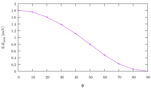
Fig. 29 Magnetization curve from Z to the X axis