Basis sets - Special cases
Do you want to get all tutorial materials on your local machine?
You can get all files and set up your local environment. Do that now before proceeding.
In this tutorial we will cover a few additional considerations on basis sets when using SIESTA, particularly in the context of the Basis Set Superposition Error and properties that require a better description of the vacuum region.
If you have not done so already, we recommend that you first read the tutorial on basis set optimization. This optimization usually comes before considering what we will cover here.
Additional information
As a general background for this topic, you can watch the 2021 talks by Emilio Artacho:
background Staring at the void: the vacuum region
Contrary to plane-wave descriptions, atomic-centered basis sets do not fill the entire space of your simulation. This is key to their efficiency, but it also means that the description of the vacuum region might be lacking in some cases. The two tricks we will be covering here (diffuse orbitals and ghost atoms) are meant to solve this issue with little effort.
Diffuse orbitals
The term diffuse orbitals refers to basis functions that have a long cut-off radius. These orbitals are added after the basis set has been optimized, and we will use an arbitrarily large cut-off radius.
So suppose we have a PAO.Basis block that looks like this for a carbon atom:
%block PAO.Basis
C       2
n=2   0   2
  0.000      0.000
  1.000      1.000
n=2   1   2 P   1
  0.000      0.000
  1.000      1.000
%endblock PAO.Basis
We have here two shells with n=2: a double-zeta s-type shell and a double-zeta p-type shell with a single polarization orbital. We can then add a diffuse orbital by adding a new shell with a higher n, for example:
%block PAO.Basis
C       3 ! Note the increase 2->3
n=2   0   2
  0.000      0.000
  1.000      1.000
n=2   1   2 P   1
  0.000      0.000
  1.000      1.000
n=3   0   1
  10.000
   1.000
%endblock PAO.Basis
Note that we used an arbitrary value for the cut-off radius, of 10 Bohr. Usually, values chosen range for 10 to 15 Bohr, depending on the system. If 10 is enough to get a given property converged, then you’re good to go!
A thing worth noting is that you can always have any amount of extra diffuse orbitals. Usually, you add diffuse orbitals until the property you want to calculate is converged enough, but a little chemical or physical intuition also helps.
Basis Set Superposition Error
A concept that is key for atomic-centered basis in general is the Basis Set Superposition Error or BSSE. All kinds of DFT codes are subject to this error, so long as they use atom-centered basis sets. The general idea is that, given an atom A, the basis functions coming from neighbouring atoms B also help improve the description of the electronic density around A. If we remove those neighbours, we effectively end up with a poorer description.
These are some examples in which BSSE is surely present:
Dimer energy calculations: we will cover this example below. Essentially, each single monomer molecule has a better numerical description in the dimer than alone.
Adsorption energy: similar to the dimer above.
Vacancy formation energy: by removing an entire atom from the system, we have effectively removed a place in space where functions from other atoms might not reach.
The better the basis set, the less important this issue becomes. However, one way to completely remove this issue in some cases is by using ghost atoms.
Ghost atoms
SIESTA can place basis orbitals anywhere, not just in the position of atoms. The main way to do this is by using ghost atoms. Ghost atoms are not real atoms, in the sense that they do not have a nuclear charge, and they do not add electrons to the system. They are just a convenient way to place basis functions in places where there are no atoms.
In order to do this in SIESTA, we just add an atom and set their atomic number to a negative value: -8, for example, will place a ghost oxygen, while -6 will place a ghost carbon (this will be detailed later). For this, you will need to generate an extra atom species in the ChemicalSpeciesLabel block.
- Ghost atoms can be useful in a variety of cases, for example:
When fixing the BSSE in dimer, binding or vacancy calculations.
To improve the treatment for the electronic density in slabs, increasing the quality of the description in the near-vacuum region.
Both of these cases will be considered below.
basic Fixing the Basis Set Superposition Error
Are you under a local environment?
Enter the directory 01-WaterDimer-BSSE
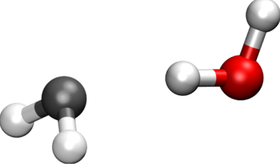
Fig. 3 A water molecule (right) with another ghost water molecule (left) to represent what we have in the dimer.
If you ran the tutorial on basis set optimization, you might have noticed that the binding energy can be twice as large as the planewaves result; at least, when choosing the default settings for SIESTA. Even for our optimized basis set, we might be up to 50 meV away from it. Is this really the best result we can get?
It just so happens that in our case, the dimer, each of the water molecules is slightly better described if we take in to account the basis functions of the other water molecule. Thus, it is as if our monomer had a poorer basis set than the dimer, and we are in a case in which the BSSE is important.
Luckily enough, there are a few ways so solve this issue, the most common one involving ghost atoms. As mentioned before, ghost atoms are just points in space in which we add basis functions that would belong to a given atom if it were there. In our case, we will turn each of the water molecules in a ghost ending up with the following systems:
Water1+ (Ghost)Water2
(Ghost)Water1+ Water2
We’ll now have a look at the input files:
Pseudos:
O.psml,H.psml,O_ghost.psml,H_ghost.psmlInput files:
monomer.fdf,dimer.fdf,ghost1.fdf,ghost2.fdf
We will use four different input files: monomer.fdf has a single water molecule, while dimer.fdf has the water dimer. ghost1.fdf and ghost2.fdf have the geometries of the dimer, but with one of the water molecules as a set of ghost atoms. Take a look, for example, at the ghost1.fdf file, you will notice a few distinct things:
14%block ChemicalSpeciesLabel
15 1  8  O
16 2  1  H
17 3 -8  O_ghost
18 4 -1  H_ghost
19%endblock ChemicalSpeciesLabel
20
21AtomicCoordinatesFormat  Ang
22%block AtomicCoordinatesAndAtomicSpecies
23 0.000000    0.000000    0.000000 4
24 0.000000    0.000000    1.522047 4
25 0.436628    0.395162    0.761024 3
26 2.341468    0.000000    0.760784 2
27 3.795635    0.459564    0.760954 2
28 3.251445   -0.331791    0.760767 1
29%endblock AtomicCoordinatesAndAtomicSpecies
Aside from the normal oxygen and hydrogen, do you see the two additional species? Note O_ghost and H_ghost, which have negative atomic numbers. This indicates that those species will be ghosts! If you look below in the coordinates, you will see that the first water molecule is the ghost (the atoms have species indexes 3 and 4).
There are two more things we have to take into account now: first, the pseudopotential files. Since these ghosts are techincally a new species, we need to have pseudos for them. So what do we do? We just copy and rename the pseudopotential files for the normal atoms. See how H.psml and H_ghost.psml are the same file?
Additional information: Reusing the same pseudopotential file.
Instead of copying and pasting the pseudopotential file with a new name, you can re-use the same file by adding an extra term to the ChemicalSpeciesLabel block:
%block ChemicalSpeciesLabel
  1  8  O
  2  1  H
  3 -8  O_ghost  O.psml
  4 -1  H_ghost  H.psml
%endblock ChemicalSpeciesLabel
In this case, O_ghost will use the O.psml file, and H_ghost will use the H.psml file.
Second, if we use the PAO.Basis block (which, we will), we also need to generate a new section for this new species!
39%block PAO.Basis
40H 1
41 n=1 0 2 P 1
42  0.0 0.0
43O 2
44 n=2 0 2
45  0.0 0.0
46 n=2 1 2 P 1
47  0.0 0.0
48H_ghost 1
49 n=1 0 2 P 1
50  0.0 0.0
51O_ghost 2
52 n=2 0 2
53  0.0 0.0
54 n=2 1 2 P 1
55  0.0 0.0
56%endblock PAO.Basis
Now that you’ve seen the important parts of it, What is the difference between ghost1.fdf and ghost2.fdf ?
Answer: Difference between ghost1.fdf and ghost2.fdf.
The only difference is in the block AtomicCoordinatesAndAtomicSpecies. For ghost2.fdf, what changes is the order of the species:
22%block AtomicCoordinatesAndAtomicSpecies
23 0.000000    0.000000    0.000000 4
24 0.000000    0.000000    1.522047 4
25 0.436628    0.395162    0.761024 3
26 2.341468    0.000000    0.760784 2
27 3.795635    0.459564    0.760954 2
28 3.251445   -0.331791    0.760767 1
29%endblock AtomicCoordinatesAndAtomicSpecies
This means that the other water molecule is the ghost.
Now for the last part of the puzzle, how do we calculate the binding energy when having ghost atoms? Remember that the original definition is:
\(E_{\rm binding} = E_{\rm dimer} - 2E_{\rm monomer}\)
But now we have two possible escenarios for a monomer with ghosts: water 1 as a ghost with water 2 as the monomer (ghost1); or water 1 as the monomer, with water 2 as the ghost (ghost2). So now, the definition of the binding energy becomes:
\(E_{\rm binding} = E_{\rm dimer} - E_{\rm ghost1} - E_{\rm ghost2}\)
Now we can run our siesta calculation as usual:
$ siesta < monomer.fdf > monomer.out
$ siesta < ghost1.fdf > ghost1.out
$ siesta < ghost2.fdf > ghost2.out
$ siesta < dimer.fdf > dimer.out
And we can get the total energy for each of the systems:
$ grep "Total =" *.out
Output
dimer.out:siesta:         Total =    -965.509762
ghost1.out:siesta:         Total =    -482.645640
ghost2.out:siesta:         Total =    -482.646198
monomer.out:siesta:         Total =    -482.594903
For this case, with 0.001 Ry, we would get a binding energy of -320.0 meV if we do not consider the BSSE, but we get -217.9 meV if we take it into account with the ghost atoms. That’s more than a 100 meV difference! This error (102.1 meV) accounts for as much as the 32% of the binding energy if we do not take it into account.
If we look in the literature for reported binding energy values for the dimer, we find a value of 228.6 meV using planewaves, which is fairly close to the value we’re finding roughly if we take BSSE into account. (Corsetti et al., 2013).
Now, try different values for the energy shift, namely 0.01 Ry and 0.0001 Ry. Compare the binding energies with and without the BSSE correction. How much of the original binding energy can be adjudicated to BSSE?
Answer: Basis enthalpy for different values of energy shift.
We have now the energies for monomer, dimer, and ghost combinations for different energy shifts:
Energy Shift      Monomer      Dimer       Ghost1        Ghost2
 0.01 Ry       -482.136281  -964.717861  -482.174049  -482.329897
 0.001 Ry      -482.594903  -965.509762  -482.645640  -482.646198
 0.0001 Ry     -482.632604  -965.578226  -482.684753  -482.671886
If we calculate the binding energies with and without BSSE correction, we should get something like this:
Energy Shift  No BSSE  With BSSE   BSSE   BSSE%
 0.01 Ry      -471.9    -213.9    -258.0   55
 0.001 Ry     -320.0    -217.9    -102.1   32
 0.0001 Ry    -313.0    -221.5     -91.5   29
Note how, with a lower energy shift (i.e., larger orbitals), we get a much lower contribution with regards to BSSE. In the highest value for energy shift, the BSSE is actually larger than the binding energy!
In general, seeing how much of BSSE is present in things like binding energy is a good indicator of how transferrable your basis set is. If you did the basis set optimization tutorial, you might want to check how each of your basis sets perform when checking for BSSE!
Remember that you will have to duplicate the sections in the PAO.Basis block for ghost1.fdf and ghost2.fdf. They should look something similar to the following block:
Optimized PAO.Basis with ghosts.
%block PAO.Basis
  H 1
    n=1 0 2 P 1
        4.5 2.0
  O 2
    n=2 0 2
        5.5 3.0
    n=2 1 2 P 1
        7.0 3.0
  H_ghost 1
    n=1 0 2 P 1
        4.5 2.0
  O_ghost 2
    n=2 0 2
        5.5 3.0
    n=2 1 2 P 1
        7.0 3.0
%endblock PAO.Basis
Answer: Basis enthalpy for optimized basis sets.
We have picked here different stages from the basis set optimization tutorial.
Basis Set    Monomer     Dimer       Ghost1       Ghost2
Default    -482.136281 -964.717861 -482.174049      -482.329897
Rough      -482.884135 -966.016972 -482.888456  -482.906653
OptimRcut  -482.936001 -966.119097 -482.941834  -482.948588
OptimPolar -482.980804 -966.205087 -482.987083  -482.986743
The Default refers to the siesta default basis set, while Rough refers to the optimization done only with PAO.EnergyShift and PAO.SplitNorm, using 0.001 Ry and 0.55 respectively. OptimRcut refers to the optimization done on cut-off and matching radii, which results in the following block:
Optimized PAO.Basis radii
%block PAO.Basis
H 1
  n=1 0 2 P 1
      4.5 2.0
O 2
  n=2 0 2
      5.5 3.0
  n=2 1 2 P 1
      7.0 3.0
%endblock PAO.Basis
Finally, OptimPolar refers to an additional optimization performed on the Polarization orbitals, resulting in this last block:
Optimized PAO.Basis radii
%block PAO.Basis
H 2
 n=1 0 2
  4.5 2.0
 n=2 1 1 Q 4.0
  4.5
O 3
 n=2 0 2
  5.5 3.0
 n=2 1 2
  7.0 3.0
 n=3 2 1 Q 6.5
  7.0
%endblock PAO.Basis
Translating these into binding energies, we get:
Basis Set  No BSSE  With BSSE    BSSE   BSSE%
Default     -445.3    -213.9    -231.4  51.96
Rough       -248.7    -221.9     -26.8  10.79
OptimRcut   -247.1    -228.7     -18.4   7.45
OptimPolar  -243.5    -231.3     -12.2   5.02
Note how the fully optimized basis sets not only reproduce the binding energy more accurately, but also the contribution of BSSE is greatly reduced. Note, also, that there is very little gain when optimizing the polarization orbitals over just optimizing the cut-off radii.
basic Basis sets for 2D materials: improving vacuum description
Are you under a local environment?
Enter the directory 02-Graphene

Fig. 4 Graphene, the quintessential 2D system.
In this example, we will illustrate the tuning of the basis set orbitals for a slab system. 2D systems in general represent a scenario in which where the vacuum must be properly described in one direction (perpendicular to the plane), specially if you want to capture specific surface-related properties. We will use graphene (the prototypical 2D system), but similar effects are important for other layered materials and surfaces (see for example García-Gil et al., 2009).
First, let’s have a look at the input files:
Pseudos:
C.psml,C_ghost.psmlInput files:
graphene.fdf,graphene.diffuse.fdf,graphene.ghosts.fdf
Note
In this section of the tutorial, we will be using gnubands and gnuplot to obtain plots of the band structure. gnubands is a utility within SIESTA, so you do not need to install anything else.
Let’s first have a look at graphene.fdf. As you can see, it is a conventional fdf file, and it doesn’t even have a PAO.Basis block (yet). The only parts that might not sound familiar are the options regarding k-point sampling and band structure output, which are covered in other tutorials (see the K-point sampling and Analysis tools tutorials).
A peek at the fdf file
 1SystemName    graphene
 2SystemLabel   graphene
 3
 4NumberOfAtoms    2
 5NumberOfSpecies  1
 6%block ChemicalSpeciesLabel
 7    1   6  C
 8%endblock ChemicalSpeciesLabel
 9
10PAO.BasisSize    DZP
11PAO.EnergyShift  300 meV
12
13# Structure
14LatticeConstant 2.476675 Ang
15%block LatticeParameters
161.000  1.000  20.0  90.0  90.0  120.0
17%endblock LatticeParameters
18
19AtomicCoordinatesFormat fractional
20%block AtomicCoordinatesAndAtomicSpecies
21  0.33333333  0.66666667  0.5        1     # C
22  0.66666667  0.33333333  0.5        1     # C
23%endblock AtomicCoordinatesAndAtomicSpecies
24
25# K-point sampling for electronic structure.
26%block kgrid_Monkhorst_Pack
27  9  0  0    0.0
28  0  9  0    0.0
29  0  0  1    0.0
30%endblock kgrid_Monkhorst_Pack
31
32# Options for bands output.
33WriteKbands        T
34WriteBands         T
35BandLinesScale     ReciprocalLatticeVectors
36%block Bandlines
37  1   0.0000000000   0.000000000   0.0000   \Gamma
38 60   0.3333333333   0.333333333   0.0000   K
39 30   0.5000000000   0.500000000   0.0000   M
40 60   0.0000000000   1.000000000   0.0000   \Gamma
41%endblock BandLines
42
43# Other options
44XC.Functional          LDA
45XC.Authors             CA
46MeshCutoff             160.0 Ry
47
48SCF.Mixer.Weight        0.1
49SCF.Mixer.History       3
50SCF.DM.Tolerance        5.0d-5
Just to characterize the problem a bit, run the graphene system varying the energy shift (PAO.EnergyShift) across 300 meV, 100 meV, 50 meV and 10 meV. Take note of the total energy and the basis enthalpy.
Remember that you can run this system as usual:
$ siesta < graphene.fdf > graphene.out
And that you can easily grep the total energy and the basis enthalpy from the output:
$ grep "E + p_basis" graphene.out
$ grep "Total =" graphene.out
Answer: Energy and Basis Enthalpy for different Energy Shifts
You should get something similar to these results:
Eshift    BasisEnthalpy    TotalEnergy
10 meV   -325.843477 eV   -326.027291 eV
50 meV   -325.992000 eV   -326.102045 eV
100 meV  -326.025687 eV   -326.111045 eV
300 meV  -325.912154 eV   -325.965841 eV
At first look, 100 meV looks like a reasonable value for the energy shift, by virtue of being a minimum of both total energy and basis enthalpy.
If we are following the same criteria as in the basis set optimization tutorial, it would seem that 100 meV is a good energy shift to get a reasonable electronic structure. So now let’s have a look at the bands.
We have here the bands obtained with a planewaves code, which we asume is a reasonable description for this kind of system:
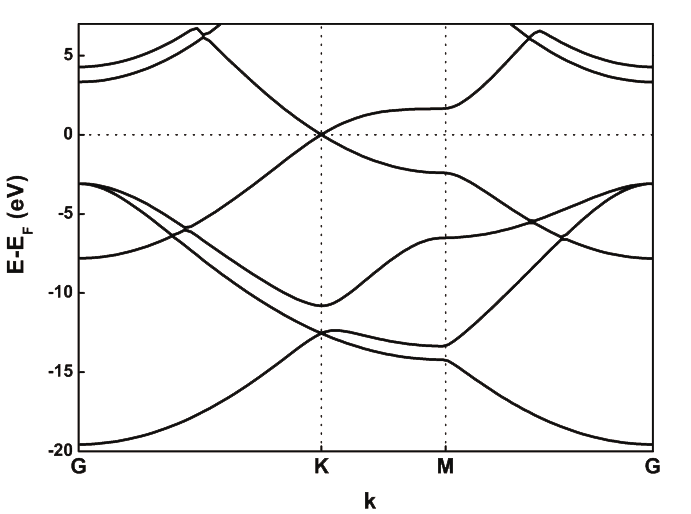
Fig. 5 Graphene band structure with VASP.
Now, let’s try to see if SIESTA produces a structure similar to the one in the picture above. We will rely on gnubands and gnuplot for this purpose:
$ gnubands -G -F -o graph -E 10 -e -20 graphene.bands
$ gnuplot --persist -e "set grid" graph.gplot
The output of gnubands is a datafile with the band structure and a graph.plot file that can be used by gnuplot. How does your band structure compare to the one obtained by planewaves?
Answer: Bands for the current basis set
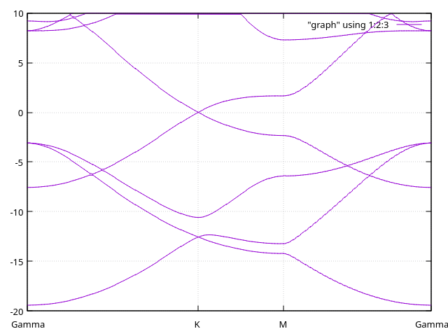
We can see that the bands that ar below the Fermi level (0 in the Y axis) are very well descripted; however, in planewaves we can see a very different structure for those bands 4-5 eV above the Fermi level (\(\sigma^*\)).
You can see that the description is not as good as we hoped for. Moreover, the patterns we see will remain for even lower values for energy shifts (i.e., longer cutoff radii). We will now see two different ways in which this problem is tackled.
Using diffuse orbitals
We can now have a look at the graphene.diffuse.fdf file.
A peek at the fdf file
 1SystemName    graphene.diffuse
 2SystemLabel   graphene.diffuse
 3
 4NumberOfAtoms    2
 5NumberOfSpecies  1
 6%block ChemicalSpeciesLabel
 7    1   6  C
 8%endblock ChemicalSpeciesLabel
 9
10PAO.EnergyShift      100.0 meV
11%block PAO.Basis
12C        4            # We include 4 shells
13 n=2   0   2          # 2s (double zeta)
14   0.000      0.000
15   1.000      1.000
16 n=2   1   2 P   1    # 2p (double zeta) + polarization (single zeta)
17   0.000      0.000
18   1.000      1.000
19 n=3   0   1          # 3s diffuse orbital (single zeta)
20  10.000
21   1.000
22 n=3   1   1          # 3p diffuse orbital (single zeta)
23  10.000
24   1.000
25%endblock PAO.Basis
26
27# Structure
28LatticeConstant 2.476675 Ang
29%block LatticeParameters
301.000  1.000  20.0  90.0  90.0  120.0
31%endblock LatticeParameters
32
33AtomicCoordinatesFormat fractional
34%block AtomicCoordinatesAndAtomicSpecies
35  0.33333333  0.66666667  0.5        1     # C
36  0.66666667  0.33333333  0.5        1     # C
37%endblock AtomicCoordinatesAndAtomicSpecies
38
39# K-point sampling for electronic structure.
40%block kgrid_Monkhorst_Pack
41  9  0  0    0.0
42  0  9  0    0.0
43  0  0  1    0.0
44%endblock kgrid_Monkhorst_Pack
45
46# Options for bands output.
47WriteKbands        T
48WriteBands         T
49BandLinesScale     ReciprocalLatticeVectors
50%block Bandlines
51  1   0.0000000000   0.000000000   0.0000   \Gamma
52 60   0.3333333333   0.333333333   0.0000   K
53 30   0.5000000000   0.500000000   0.0000   M
54 60   0.0000000000   1.000000000   0.0000   \Gamma
55%endblock BandLines
56
57# Other options
58XC.Functional          LDA
59XC.Authors             CA
60MeshCutoff             160.0 Ry
61
62SCF.Mixer.Weight        0.1
63SCF.Mixer.History       3
64SCF.DM.Tolerance        5.0d-5
The file graphene.diffuse.fdf includes 3s and 3p orbitals with very long tails. These are enough to lower the energy of the \(\sigma^*\) states below 5 eV. You can see these orbitals in the PAO.Basis block section of the input:
11%block PAO.Basis
12C        4            # We include 4 shells
13 n=2   0   2          # 2s (double zeta)
14   0.000      0.000
15   1.000      1.000
16 n=2   1   2 P   1    # 2p (double zeta) + polarization (single zeta)
17   0.000      0.000
18   1.000      1.000
19 n=3   0   1          # 3s diffuse orbital (single zeta)
20  10.000
21   1.000
22 n=3   1   1          # 3p diffuse orbital (single zeta)
23  10.000
24   1.000
25%endblock PAO.Basis
Note that the carbon atom now has four shells (C 4). We add both s and p
orbitals as diffuse since we expect both to participate in a \(\sigma^*\)
band!
Run the graphene.diffuse.fdf file and compute the bands (you will now have to use gnubands with graphene.diffuse.bands). Repeat the calculation, but increasing the cut-off radii of the diffuse orbitals to 12 Bohr. How do the bands behave?
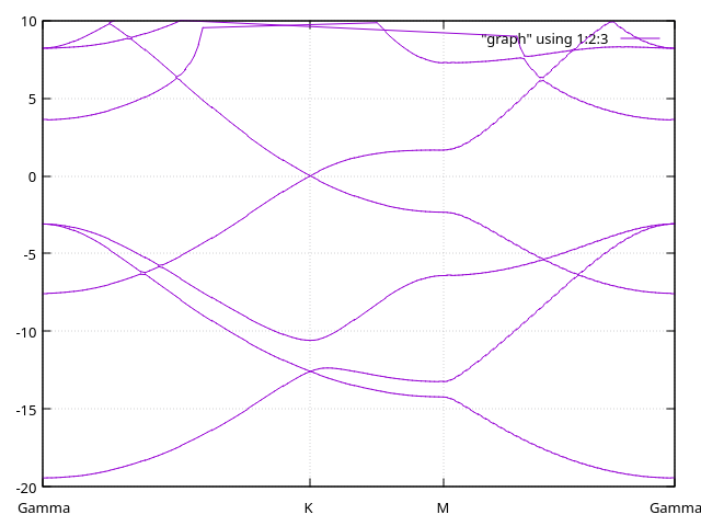
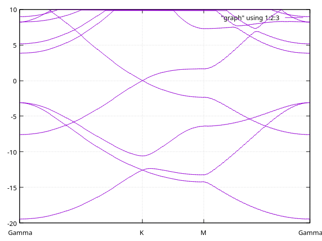
Answer: Bands with diffuse orbitals.
We have here the bands with 10 Bohr-long diffuse orbitals.
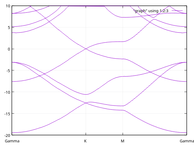
And here, the bands with 12 Bohr-long diffuse orbitals:

Additional information: Using only S diffuse orbitals.
In case you are wondering what happens if you only add a single diffuse S orbital, you can see the bands here:
Only the first of the \(\sigma^*\) is affected. To fully capture the correct band structure, we need the p orbitals indeed.
We can see in this case that adding diffuse orbitals solves our problem. But we still have another way to fix this… using ghost atoms again!
Using ghost atoms
How do we use ghost atoms to solve the same problem? Let’s have a look at the graphene.ghosts.fdf file. In particular, the lines on species and geometry:
 8%block ChemicalSpeciesLabel
 9    1   6  C
10    2  -6  C_ghost  # Ghost species!
11%endblock ChemicalSpeciesLabel
23%block AtomicCoordinatesAndAtomicSpecies
24  0.33333333  0.66666667  0.5        1     # C
25  0.66666667  0.33333333  0.5        1     # C
26  0.33333333  0.66666667  0.55       2     # Ghost-C above
27  0.66666667  0.33333333  0.55       2     # Ghost-C above
28  0.33333333  0.66666667  0.45       2     # Ghost-C below
29  0.66666667  0.33333333  0.45       2     # Ghost-C below
30%endblock AtomicCoordinatesAndAtomicSpecies
You can see that it includes a layer of ghost orbitals (C ghosts) slightly above and below the graphene plane. By doing this we are able to describe electronic states that extend farther away from the atomic layer into the vacuum (at the cost of including a significant number of orbitals in the basis).
Note
We use here the same carbon atoms as ghosts for convenience, but we are not aiming to correct BSSE here! Your ghost atoms could be of any other type, you could have for example ghost hydrogens, or sulfur, or whatever atom you want.
Run the graphene.ghosts.fdf file and compute the bands (you will now have to use gnubands with graphene.ghosts.bands). How do the bands compare to the cases before?
Answer: Bands with ghost atoms.
We have here the bands with ghosts atoms on top of the surface.
Diffuse orbitals versus Ghosts
You have a summary of the comparisons in the following image:
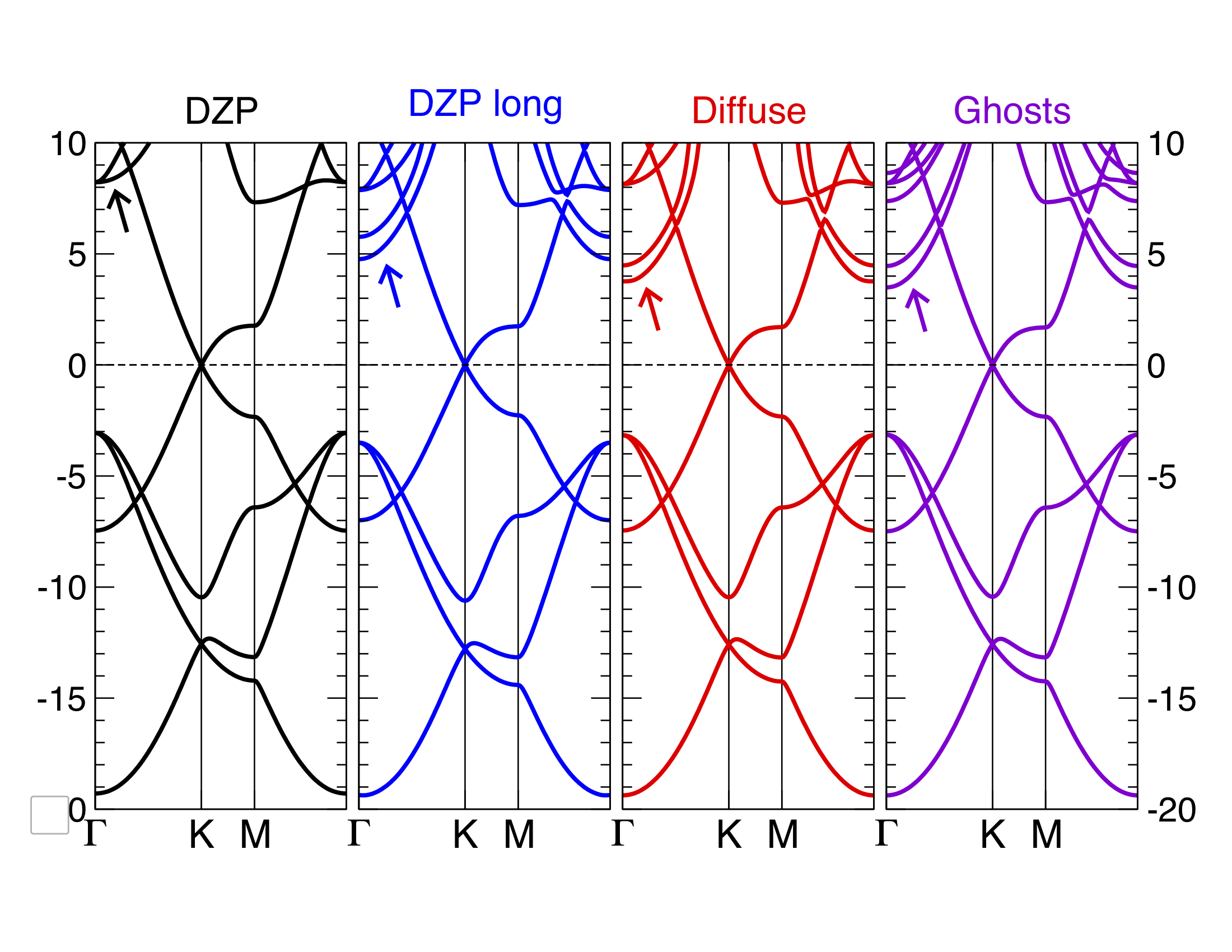
Fig. 6 Graphene bands with SIESTA with various basis sets.
The “DZP long” part refers to a normal DZP basis set but with extremely long cut-off radii. You can see that both the ghost atoms and the diffuse orbitals are good solutions, but which one would you pick? For your own systems, consider the following:
Which of the approaches adds more basis functions to the system? How does this reflect on the total computational time?
Which of the approaches makes more sense for the technique you are using? Using ghost atoms is perfectly fine for RT-TDDFT, but it’s not ideal for molecular dynamics, for example.
If you are using ghost atoms, where do you place them? And do you use the same atoms as in the surface? Or a different atom for the ghosts?
If you use diffuse orbitals, do you apply the diffuse orbital to all atoms of the same species? Or do you create a specific atomic species only for those atoms on the surface?