Sampling of the BZ with k-points
Do you want to get all tutorial materials on your local machine?
You can get all files and set up your local environment. Do that now before proceeding.
In this exercise we will explore the convergence with k-point sampling for a (semi)metalic system, and compare it with an insulator. We have selected three carbon-structures that are particularly easy to converge in terms of basis and real-space mesh. You will work in the directories graphene (basic), graphite, and diamond (advanced.
background K-point sampling
K-points (or k-vectors) are fundamental concepts in periodic electronic structure calculations that deal with crystalline materials. They represent the discrete points used to sample the Brillouin Zone (BZ), which is the unit cell (e.g. space that contains all unique and physically distinct k-vectors) of the reciprocal lattice. The crystal’s total energy, charge density, and electronic band structure are calculated at these selected k-points.
The k-point sampling density determines how well discrete sums approximate continuous BZ integrals. All properties of the crystal, such as the total energy and charge density, are found by integrating over the entire BZ. Therefore, accurate integration over the BZ is essential.
Too coarse sampling leads to:
Errors in total and relative energies
Shifts, instabilities and general inaccuracies at and around the Fermi level
Poor density of states (DOS) representation (spikes, missing features)
Metals and semimetals are especially challenging, since small changes in sampling can drastically alter occupations. This tutorial shows how to systematically test convergence with respect to k-point sampling.
Hint
This method works for both 2D and 3D periodic systems. For slab or vacuum systems, sampling is generally only needed in the periodic directions.
basic Testing kpoint-convergence with Energy
Hint
Enter the 01-Graphene directory, and complete the basic exercises. The advanced ones will consist in replicating the same for the 02-Diamond and 03-Graphite directories.
In this section, we examine the differences in setting the k-point sampling for two carbon polymorphs: graphene as a representative 2D structure and diamond as a 3D one.
Using kgridcutoff
The kgridcutoff parameter is used to automatically generate an appropriate
k-point grid based on a desired real-space resolution.
It defines a maximum desired resolution in real space, and SIESTA translates
this requirement into a minimum number of k-points needed to sample the BZ.
The larger the value of kgridcutoff, the finer the sampling in reciprocal space.
Begin the exercise by uncommenting the kgridcutoff line and assigning it a value,
for example:
kgridcutoff 4 bohr
Then, examine the following useful information from the output:
The effective k-cutoff:
siesta: k-cutoff (effective) = 2.477 Ang
Total number of k-points:
siesta: k-grid: Number of k-points = 2
k-points sampling in each direction of the reciprocal space:
siesta: k-grid:     0     2     0      0.500
siesta: k-grid:     2     0     0      0.500
siesta: k-grid:     0     0     1      0.000
Now, rerun the calculation using the modified fdf files for graphene, using kgridcutoff = 10.0, 20.0, 30.0 bohr, and record the effective k-cutoff, number of k-points, and energy.
Explicit Monkhorst–Pack grids
Now we will illustrate the explicit k-point information generated
when using a Monkhorst–Pack grid in a calculation.
Activating the WriteKpoints True option results in a detailed list showing
each k-point’s coordinates and weight for Brillouin zone sampling.
The same information is included in the SystemLabel.KP file:
siesta: k-point coordinates (Bohr**-1) and weights:
siesta:            1  0.149858E+00  0.149858E+00  0.149858E+00   0.250000E+00
siesta:            2  0.449573E+00 -0.149858E+00 -0.149858E+00   0.250000E+00
siesta:            3 -0.149858E+00  0.449573E+00 -0.149858E+00   0.250000E+00
siesta:            4  0.149858E+00  0.149858E+00 -0.449573E+00   0.250000E+00
Each k-point is assigned a weight, which represents the volume of the BZ that the k-point is assumed to represent in the discrete sum. The distribution of the k-points is set in line with the geometry of the input system.
To manually set the kgrid sampling, comment out kgridcutoff and uncomment
the block kgrid_Monkhorst_Pack (a systematic way to sample BZ with uniform meshes)
in both fdf files:
%block kgrid_Monkhorst_Pack
4 0 0  0.5
0 4 0  0.5
0 0 1  0.0
%endblock kgrid_Monkhorst_Pack
Compare the number of used k-points with the previous case. Create a table summarizing your results like this:
k-grid |
# of k-points |
Energy (eV) |
ΔE (meV) |
|---|---|---|---|
4×4×1 |
… |
… |
… |
6×6×1 |
… |
… |
… |
8×8×1 |
… |
… |
… |
12×12×1 |
… |
… |
… |
16×16×1 |
… |
… |
… |
20×20×1 |
… |
… |
… |
24×24×1 |
… |
… |
… |
Note
To ensure convergence of the kgrid, monitor changes in the total energy of the system. Compare the values retrieved from both samplings. Note that metallic systems usually require a large number of k-points to converge.
basic K-point convergence with bands and DOS
Here we will focus on the Density of States (DOS) for graphene. For that, we
will need to edit graphene.fdf to use a 4x4x1 grid:
%block kgrid_Monkhorst_Pack
4  0  0    0.5
0  4  0    0.5
0  0  1    0.0
%endblock kgrid_Monkhorst_Pack
Run the scf cycle as usual. As we will see, this is insufficient for a good description of graphene.
To plot the DOS we will use the utility program Eig2DOS. For the broadening
for each state in eV a value of the order of the default (0.2 eV) is usually
reasonable, but if you want to reproduce the smooth V-shape close to graphene’s
Dirac cone you will probably have to decrease that value. We can try:
Eig2DOS -f -s 0.1 -n 400 -m -12.0 -M 2.0 -k graphene.KP graphene.EIG > dos
which will compute the DOS in the (12 eV, 2 eV) range around the Fermi level
(-f option), using a grid of 400 points and a broadening of 0.1 eV.
The content of the dos file can be plotted using gnuplot:
gnuplot
plot "dos" u 1:4 with lines
We get a set of spikes, with just some inkling that there might be a V-shaped feature near the Fermi level. Obviously the sampling is not good enough.
The file graphene.fdf will also produce a file graphene.bands containing the
band structure along the several lines in the Brillouin zone (BZ). This is activated by
uncommenting the following block:
%block Bandlines
  1   0.5000000000   0.000000000   0.0000   M
 30   0.0000000000   0.000000000   0.0000   \Gamma
 45   0.3333333333   0.333333333   0.0000   K
 30   0.5000000000   0.500000000   0.0000   M
%endblock BandLines
To plot the band structure we use the utility program gnubands, taking
advantage of some new features (type gnubands -h for a list of options):
gnubands -F -G -o bandstructure -E 10 -e -20 *.bands
That will shift the origin of energy to the Fermi level. With the above command we will get a window between -20 eV and 10 eV with respect to EF. Also, a ‘bandstructure.gplot’ driver file is created automatically (which has extra information to place and label the ‘ticks’ for each symmetry point in the BZ). Now we plot:
gnuplot --persist -e "set grid" bandstructure.gplot
The position of the Dirac cone is highlighted by the gridline passing by the high-symmetry K point). It is obvious, however, by looking at the EF gridline, that the Fermi level does not fall exactly at the Dirac cone, as it should (see Fig. 7).
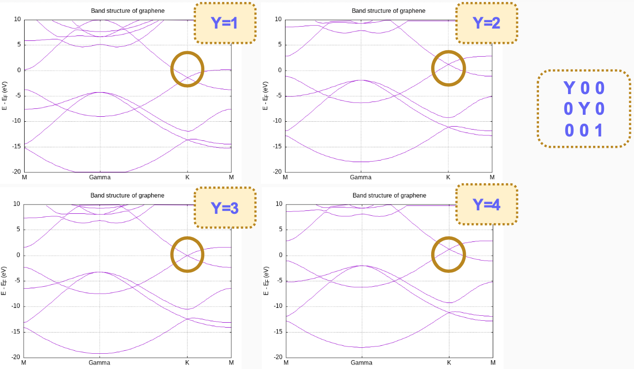
Fig. 7 Graphene band structure for increasing Monkhorst-Pack grids.
The position of the Fermi level in (semi)metals is very sensitive to the k-point mesh used. In this case, the 4x4x1 sampling originally set in the input file is clearly not appropriate. You can increase the Monkhorst-Pack parameters and check the convergence. Notice also that in graphene (and other hexagonal lattices) the K-point (1/3,1/3,0) is particularly relevant, and it is advisable that it is explicitly included in the discretization. In fact, in this case including the K-point makes all the difference, as can be seen by using this block:
%block kgrid_Monkhorst_Pack
 6  0  0    0.0
 0  6  0    0.0
 0  0  1    0.0
%endblock kgrid_Monkhorst_Pack
The Fermi level is now exactly at the vertex of the Dirac cone. This is not really a consequence of having increased the density of k-points, but of including the K-point in the sampling (check the graphene.KP file; note that the k-points are given in cartesian coordinates, not relative to the reciprocal basis vectors). In fact, if we use the block:
%block kgrid_Monkhorst_Pack
 3  0  0    0.0
 0  3  0    0.0
 0  0  1    0.0
%endblock kgrid_Monkhorst_Pack
Leading to a much coarser sampling, we still get the Fermi level correctly aligned. The presence of the K point in the sampling set pins the Fermi level at the Dirac cone.
It is also instructive to see the behavior of the DOS when the k-point sampling gets more dense. For coarse samplings, it does not look at all like the “free-electron-like” curve we see in textbooks. This is due to the very simple method used to construct the DOS (just broadening a collection of discrete energy levels). You probably have to increase the mesh beyond 60x60x1 to have good plots for the DOS.
Note
You do not need to run again a full scf cycle to get the DOS with more
k-points. You could re-use the converged density-matrix to shorten the cycle
(option DM.UseSaveDM). There is an alternative route that does not use
the .EIG file, but the computation of the partial density of states. Just
include the blocks:
%block ProjectedDensityOfStates
  EF -20.00  10.00  0.100  500  eV
%endblock ProjectedDensityOfStates

%block PDOS.kgrid_Monkhorst_Pack
 60  0  0    0.0
 0  60  0    0.0
 0   0  1    0.0
%endblock PDOS.kgrid_Monkhorst_Pack
and the program will compute the pDOS (and the DOS) in a finer grid. The DOS is in graphene.DOS, which can be plotted as:
gnuplot> plot "graphene.DOS" u 1:2 with lines
to get a figure similar to Fig. 8. (Note that the scf sampling was set to 6x6x1, as above). The pDOS information might be useful.
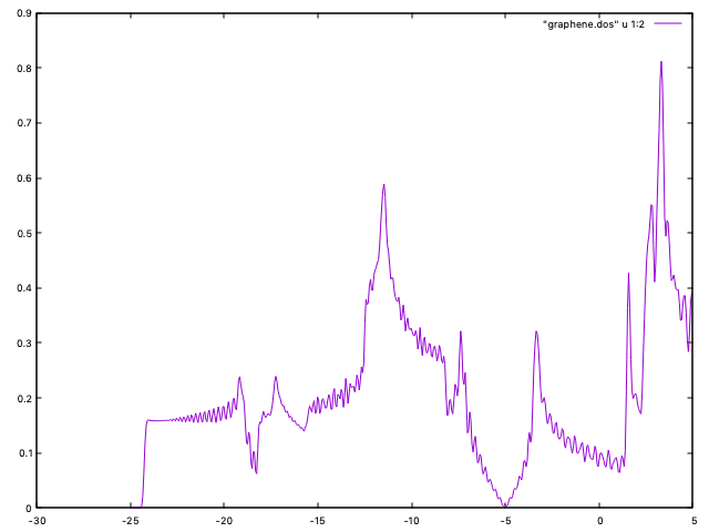
Fig. 8 Graphene DOS (60x60x1 k-sampling)
intermediate Computational time vs k-point sampling
Repeat the previous exercise, but now measure the computational time as a
function of the k-point sampling. You can use either kgridcutoff or
kgrid_Monkhorst_Pack. Try to cover a wide range of k-point densities,
from very coarse to very fine, and compare how this fine-tuning affect the time to
solution compared to other input values (i.e. mesh cut-off). The ultimate objective is
to find the ideal setup that gives accurate results at the minimal computational cost.
advanced Repeat previous exercises for Diamond and Graphite
Diamond
Hint
Enter the 02-Diamond directory.
Diamond is now used as an example of a 3D periodic material.
It has fcc structure and the high-symmetry k-points points are included in the
input file diamond.fdf.
Unlike graphene and graphite, diamond is non-metallic, and the
k-point convergence is easier. Plot bands, and DOS and check the results.
Graphite
Hint
Enter the 03-Graphite directory.
Graphite is the 3D version of graphene. It is a semimetal, and similar caveats than graphene apply. Now, however, the k-point sampling along the three spatial directions must be considered.
The input graphite.fdf includes the bandlines required to plot the bands.
Notice that there is a flat band right at the Fermi level (compare with
Fig. 9). Check the convergence of the Fermi level, and the
DOS as a function of the k-sampling.
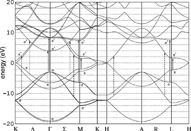
Fig. 9 Graphite bands
- For each run, record:
Total wall time
SCF iterations
Number of k-points
- Plot:
Energy error vs # of k-points
CPU time vs # of k-points
Expect diminishing returns: beyond some density, energy changes little, cost still grows.
Hint
Improving Convergence with Electronic Temperature
For metallic or semimetallic systems like graphene and graphite, achieving stable
and quick convergence for the total energy and Fermi level can be challenging,
even with a very dense k-point mesh.
In addition to fine-tuning the k-point grid, you can use the ElectronicTemperature
parameter.
This smears the electron occupation around the Fermi level, which smoothens the
integrals over BZ and can significantly improve SCF convergence and reduce oscillations
in the total energy.
Keep in mind that using a non-zero electronic temperature introduces a small
entropic free energy term in the total energy.
More information about convergence in DFT calculations, including detailed benchmarks
with SIESTA and many other DFT codes, can be consulted from a recent paper in
Nature Reviews Physics 6 (2024) 45–58.