Basis sets - Tips and tricks
Note
As a general background for this topic, you can watch the 2021 talks by Emilio Artacho:
In this tutorial we will cover a few additional considerations on basis set when using SIESTA.
Basis set generation and adjacent concepts
Basis set optimization
Best results are obtained when using an optimized basis set. See the corresponding tutorial for an example of a basis set optimization procedure.
Basis Set Superposition Error
A concept that is key for atomic-centered basis in general is the Basis Set Superposition Error or BSSE. All kinds of DFT codes are subject to this error, so long as they use atom-centered basis sets. The general idea is that, given an atom A, the basis functions coming from neighbouring atoms B also help improve the description of the electronic density around A. If we remove those neighbours, we effectively end up with a poorer description.
The better the basis set, the less important this issue becomes. However, one way to completely remove this issue in some cases is by using ghost atoms.
Ghost atoms
SIESTA can place basis orbitals anywhere, not just in the position of atoms.
In order to do this, we just place an atom and tell SIESTA that their atomic
number is negative: -8, for example, will place a ghost oxygen, while -6 will
place a ghost carbon (this will be detailed later). For this, you will need to
generate an extra atom species in the ChemicalSpeciesLabel block.
- Ghost atoms can be useful in a variety of cases, for example:
When fixing the BSSE in dimer, binding or vacancy calculations.
To improve the treatment for the electronic density in slabs, increasing the quality of the description in the near-vacuum region.
Both of these cases will be considered below.
Visualizing Orbital Shapes
You can look at the shape of the orbitals by plotting the contents of the .ion files produced by SIESTA, as explained in this how-to.
Basis sets for molecules - BSSE
Hint
Enter the directory waterDimer-BSSE
If you ran the tutorial on basis set optimization, you might have noticed that the binding energy can be twice as large as the planewaves result; at least, when choosing the default settings for SIESTA. Even for our optimized basis set, we might be up to 50 meV away from it. Is our basis set that bad?
It just so happens that in our case, the dimer, each of the water molecules is slightly better described if we take in to account the basis functions of the other water molecule. Thus, it is as if our monomer had a poorer basis set than the dimer, and we are in a case in which the BSSE is important.
Luckily enough, there are a few ways so solve this issue, the most common one involving ghost atoms. As mentioned before, ghost atoms are just points in space in which we add basis functions that would belong to a given atom if it were there. In our case, we will turn each of the water molecules in a ghost ending up with the following systems:
Water~1~ + (Ghost)Water~2~
(Ghost)Water~1~ + Water~2~
In terms of “true” atoms, each of those systems is a water monomer, but each have the additional basis functions that would correspond to the other water molecule if it were there. Thus, both systems have the same coordinates as the water dimer. Now, our binding energy becomes:
E~binding~ = E~dimer~ - E~ghost1~ - E~ghost2~
Try different values for the energy shift (0.01 Ry, 0.001 Ry and 0.0001 Ry) in *ghost1.fdf*, *ghost2.fdf*, *monomer.fdf* *dimer.fdf*, and see how the binding energies change when compared to just doing Edimer - 2*Emonomer. If you ran the tutorial on basis set optimization, you can copy your optimized PAO.Basis block into those files; in the cases where ghosts are present, rembember to copy the same basis sets to the ghost species.
Are our binding energies now closer to the planewaves result? How much of our original binding energy can be attributed to the BSSE? If you ran an optimized basis set, what are the differences between the optimized basis set and the default ones?
Basis sets for crystals
Hint
Enter the si directory
In this brief example, we will see the influence of the basis set generation in crystalline systems.
Compare the total energy, computational time, and band structure when using SZ, SZP, DZP, and TZP basis sizes. Then, for DZP, modify the value of PAO.EnergyShift until you get a reasonably converged energy.
Think about previous examples in other tutorials, in particular the energy shift convergence in methane and what you might have experienced with water. In general, the convergence of the cut off radii (or the energy shift) in bulk systems is much faster than in isolated molecules, since the basis does not need to reproduce the exponential decay of the electron density into vacuum. Thus, basis orbitals optimized for these systems tend to be shorter.
Basis sets for 2D materials
Hint
Enter the graphene directory
In this example, we will illustrate the optimization of the range of the basis set orbitals for a slab system (in the limit of ultrathin slabs, such as monolayers). As you previously stated, the convergence with respect to basis set range is much faster in bulk than in molecules. 2D systems, however, represent an intermediate scenario, where the vacuum must be properly described in one direction (perpendicular to the plane).
We will check these effect using graphene (the prototypical 2D system), but similar effects are important for other layered materials and surfaces [see for example S. Garcia-Gil et al Phys. Rev. B 79, 075441 (2009)].
The input file graphene.auto.fdf contains the required information when using the automatic basis set generation.
Compare the total energy, computational time, and band structure when using SZP, DZP, and TZP basis sizes.
Hint
To plot band structures you can use the following recipe. Let’s assume that you are trying a SZP basis set. After you run the program, type:
gnubands -G -F -o SZP -E 10 -e -20 graphene.bands
gnuplot --persist -e "set grid" SZP.gplot
The first line will create the SZP.gplot (plot script) and SZP (data) files. The second line will plot the band-structure. The label SZP is arbitrary, but if you choose it wisely for each case you try you will have easy access to the data later on.
Once we have a good basis (let’s assume that DZP satisfies our expectations),
we proceed to optimize the cutoff radii (file graphene.fdf). Instead of fully
optimizing the basis set, we will just explore the effect of
PAO.EnergyShift.
For DZP, modify the value of PAO.EnergyShift until you get a reasonably converged energy.
An optimal value should be around 100 meV. However, inspection of the bandstructure reveals that the \(\sigma^*\) bands are not properly described. These bands are ~8 eV above the Fermi level, while plane-wave calculations give energies of 4-5 eV (see Fig. 1 as a reference).
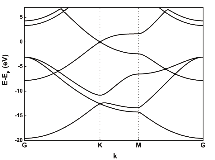
Fig. 1 Graphene band structure with VASP
You can improve the description of these states by increasing the cutoff radii
by hand in the PAO.Basis block in graphene.fdf. However, even using
orbitals with very long (and expensive) tails (up to 14 Bohrs), the description
of these bands is not accurate.
Diffuse orbitals and ghosts
You can improve further the basis set using diffuse or ghosts orbitals.
The file graphene.diffuse.fdf includes 3s and 3p orbitals with very long tails.
These are enough to lower the energy of the \(\sigma^*\) states below 5eV.
You can see these orbitals in the PAO.Basis block section of the input:
%block PAO.Basis
C       4                # We include 4 shells
n=2   0   2              # 2s orbitals (double zeta)
  0.000      0.000
   1.000      1.000
n=2   1   2 P   1        # 2p orbitals (double zeta) + polarization (single zeta)
  0.000      0.000
   1.000      1.000
n=3   0   1   # 3s diffuse orbital (single zeta) with fixed radii at 10 a.u.
  10.000
   1.000
n=3   1   1   # 3p diffuse orbital (single zeta) with fixed radii at 12 a.u.
  12.000
   1.000
%endblock PAO.Basis
Note that the carbon atom now has four shells (C 4).
Run the graphene with diffuse orbitals trying different cut-off radii for the additional diffuse orbitals (10, 12 and 14 Bohr).
Alternatively, the file graphene.ghosts.fdf includes a layer of ghost orbitals (C ghosts) slightly above and below the graphene plane. By doing this we are able to describe electronic states that extend farther away from the atomic layer into the vacuum, at the cost of including a significant number of orbitals in the basis.
Run the graphene with ghost atoms on the surface.
You can compare your results with Fig. 2.
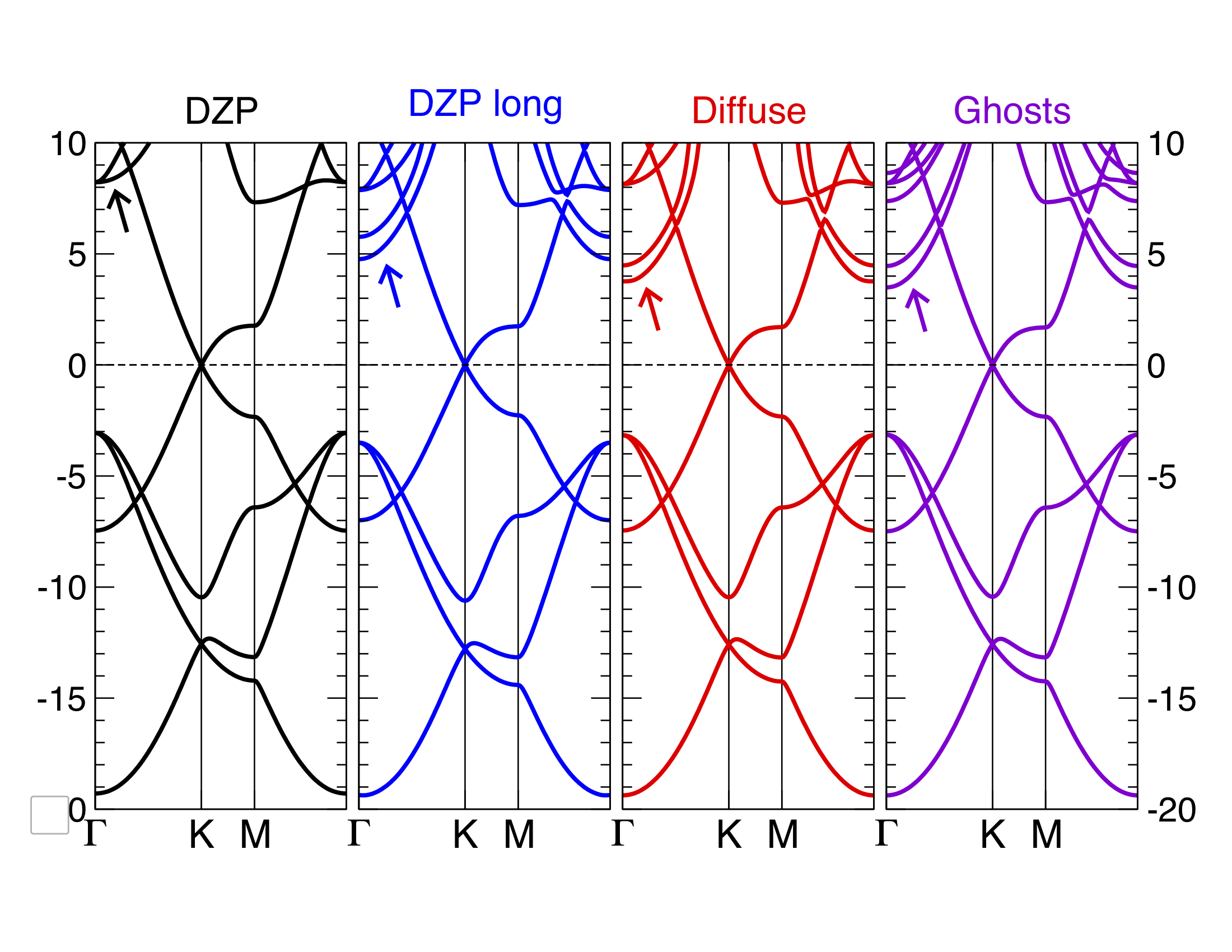
Fig. 2 Graphene bands with Siesta with various basis sets
You can try different types of basis also for the ghost orbitals and check the
results. The file GC.psf is a copy of C.psf, and is used to generate the
basis of the ghost atom, which must be defined in the ChemicalSpecies block
(with a negative Z; see the manual for details). You can use other type of
chemical species to define the ghosts.
Additional remarks
Pre-packaged basis sets
This is actually a very useful feature: if you have already generated (by
whatever means) a basis set that complies with the requirements of
Siesta (i.e., each orbital is the product of a strictly localized
radial function and a spherical harmonic), you can tabulate the radial
part and package it into a .ion file of the kind produced by
Siesta. Then, you just need to use the option:
User.Basis T
to have the program read the basis set, skipping any other internal
generation step. Actually, the .ion file contains also
pseudopotential information (via Kleinman-Bylander projectors and the
neutral-atom potential) which should be consistent with the
orbitals.
Note that there must be .ion files for all the species in the calculation. If you have them, there is no need for pseudopotential files either. (Except for DFT+U calculations, which need to generate their ‘projectors’ using the pseudopotential file)
The content of .ion files can be visualized with the tools mentioned in this how-to.