Basis sets
In this exercise we will look more closely at the basis sets used in Siesta.
Note
The required background consists of the talks by Emilio Artacho on the subject in the 2021 Siesta School:
Generalities
Pre-packaged basis sets
This is actually a very useful feature: if you have already generated (by
whatever means) a basis set that complies with the requirements of
Siesta (i.e., each orbital is the product of a strictly localized
radial function and a spherical harmonic), you can tabulate the radial
part and package it into a .ion file of the kind produced by
Siesta. Then, you just need to use the option:
user-basis T
to have the program read the basis set, skipping any other internal
generation step. Actually, the .ion file contains also
pseudopotential information (via Kleinman-Bylander projectors and the
neutral-atom potential) which should be consistent with the
orbitals.
Note that there must be .ion files for all the species in the calculation. If you have them, there is no need for pseudopotential files either. (Except for DFT+U calculations, which need to generate their ‘projectors’ using the pseudopotential file)
The content of .ion files can be visualized with the tools mentioned in this how-to.
Overview of basis-set generation options
Simple options
Siesta offers many options for the specification of the basis set. Two of the key concepts are the cardinality of the set and range of the orbitals, which can be specified, in most cases, simply with a couple of lines. For example:
PAO.basis-size DZP
PAO.energy-shift 0.01 Ry
(Recall that the energy-shift is a physical concept determining the increase in energy brought about by the confinement of the orbital, as explained in the lecture.). There are one-line options like these covering parameters such as the split-norm fraction, the soft-confinement potential, etc.
One can get quite far in the process of basis selection for a given
problem with one-line options like the above. See directory water-simple
for an example on water to explore.
The PAO.Basis block
When we specify an option such as DZP for the cardinality of the
basis set, Siesta uses internal heuristics to decide which orbitals
are actually needed, which ones to treat as ‘polarization orbitals’,
etc. For this, it uses information about the ground-state of the
element involved (stored in tables in the program code) and about the
core/valence split of the pseudopotential. Most of the time, the
heuristics work very well, but in certain cases one might need fuller
control over the specification of the orbitals. Also, sometimes it is
needed to set different values of certain parameters for different
species in the calculation. All this can be done through the
PAO.basis block. For example, the block:
%block PAO.Basis
O     2
n=2    0    2  S 0.15
  0.0  0.0
  1.0  1.0
n=2    1    3  S 0.18  P 1
  0.0   0.0   0.0
  1.0   1.0   1.0
H     1
n=1    0    2  S 0.25  P 1
  0.0   0.0
  1.0   1.0
%endblock PAO.Basis
says that O should have a ‘double zeta’ 2s shell, a ‘triple zeta’ 2p shell, and that the latter should be polarized by an extra shell. The block specifies also the ‘split-norm’ parameters to be used on a shell-by-shell basis. For H, there is a double-zeta 1s shell, polarized, and a requested value for the split norm. Note that the radii of the orbitals are set to zero. This means that the program will use any other information (in this case the split-norm values) to determine them.
The PAO.basis block can contain a very large number of
options. These are explained in the manual.
In what follows we present just a few examples of uses of the PAO.Basis blocks for cases of interest.
Ghost orbitals
Siesta can place basis orbitals anywhere, not just in the position of atoms. This is useful in certain cases. For example, in the treatment of surfaces it is sometimes necessary to provide increased variational freedom to the near-vacuum region, beyond the range of a typical orbital. In this case one can define an extra layer of ‘ghost atoms’ just outside the slab, carrying orbitals. We will see this in action in the section on basis set issues for 2D materials.
Another example is the treatment of certain defect systems, such as vacancies.
Basis optimization
The Siesta distribution contains the directory Util/Optimizer with code and examples of a framework that can be used in particular to optimize basis sets. A full treatment is beyond the scope of this simple tutorial, but the framework can be easily obtained and set up.
Case studies
Basis sets for molecules
Hint
Enter the directory h2o
This exercise is based on the H2O molecule. You will first use standard basis sets generated by SIESTA, and then a basis set specifically optimized for the H2O molecule. The ‘tips’ at the end of this text will help you in analyzing the results of the calculations.
Standard basis sets
You will find three directories: SZ, DZ and DZP, in which you will find input files for a H2O molecule, which will be solved with three different basis sets: single-Z, double-Z and double-Z plus polarizarion, respectively. The runs will consist in structural relaxations via Conjugate gradients, to find the equilibrium structure of the molecule for each of the bases used.
The bases are defined through lines like these:
PAO.BasisSize DZP
PAO.EnergyShift 500.0 meV
PAO.Splitnorm 0.15
where the first one defines the number of orbitals in the basis set (in this case, a double-Z plus polarization, which means two shells of s orbitals, two shells of p orbitals, and a polarization shell of d orbitals for oxygen, and two shells of s orbitals and one shell of polarization p orbitals for H); the second line indicates the energy shift parameter, that determines the cutoff radius of each of the orbitals; and the third one is the Split norm parameter, which defines the radius of the second-Z orbital in the case of double-Z bases.
You should do runs for each of the basis sets, changing the
PAO.EnergyShift parameter, and look at the results as a function of
basis size and localization radius (or energy shift). In particular,
you should look at:
Total energy
Bond lenghts at the relaxed structure
Bond angles at the relaxed structure
CPU time
Radius of each of the orbitals
Shape of the orbitals
You have some files with results that you should be able to reproduce in the Out directories.
Try to answer these questions:
What is the best basis set that you have found? Why?
How do the results compare with experiment?
What do you consider a reasonable basis for the molecule, if you need an accuracy in the geometry of about 1%??
In order to assess convergence with respect to basis set size, should you compare the results with the experimental ones, or with those of a converged basis set calculation?
Note
One should note that H2O is a polar molecule. Since we are using periodic boundary conditions, there is an extra non-negligible interaction with the periodic images that distorts the molecule. See the mention in the ‘first-encounter’ tutorial.
Optimized basis sets
You will now do the same calculations, but now using a basis set specifically optimized for the H2O molecule. You can find the files in directory DZP-opt.
Read the block which defines the basis set. Compare the parameters with those of the calculations in Part 1.
Do the runs with this basis set, and compare the results with the previous ones.
Tips:
Tip 1.: To find the bond lenghts, you can look in the files with extensions .BONDS or .BONDS_FINAL.
Tip 2.: You can see the radii of the orbitals in the output file, just after the line reading:
printput: Basis inputTip 3.: You can look at the shape of the orbitals by plotting the contents of the .ion files produced by Siesta, as explained in this how-to.
Basis sets for crystals
In the bulk, the convergence with respect to basis set range is much faster than in molecules, since the basis does not need to reproduce the exponential decay into vacuum.
Hint
Enter the si directory
We will illustrate this with a the very simple case of bulk Si, in order not to worry too much about other things like k-point sampling.
Start by editing the si.fdf file to select the cardinality of the basis set (SZ, DZ, SZP, DZP, etc) and check the results for the total energy.
Now, focus on the range of the orbitals by changing the
PAO.energy-shift parameter. You will find that the energy
is lowest for a particular value of that parameter, and that further
increase in the orbital range actually increases the energy.
You can also experiment by changing the range of the orbitals shell by shell, using the PAO.Basis block.
Basis sets for 2D materials
This exercise is intended to illustrate the optimization of the range of the basis set orbitals for a slab system (in the limit of ultrathin slabs, such as monolayers). As you have seen in other examples, in the bulk, the convergence with respect to basis set range is much faster than in molecules, since the basis does not need to reproduce the exponential decay into vacuum. 2D systems represent an intermediate scenario, where the vacuum must be properly described in one direction (perpendicular to the plane).
We will check these effect using graphene (the prototypical 2D system), but simular effects are important for other layered materials, and even for surfaces [see for example S. Garcia-Gil et al Phys. Rev. B 79, 075441 (2009)].
Hint
Enter the graphene directory
1. First, check the automatic basis generation, using SZ, SZP, DZ, DZP, TZ and TZP orbitals. The input file graphene.auto.fdf contains the required information. Compare the bandstructures, the total energy and the computational time for each basis. You can search for the time spent in the first SCF step:
$ grep IterSCF  graphene.out

timer: Routine,Calls,Time,% = IterSCF        1       0.151  40.55
The second to last column is the time in seconds. In this way, the computing time can also be considered in the decision of which basis is more appropriate for your study.
Hint
To plot band structures you can use the following recipe. Let’s assume that you are trying a SZ basis set. After you run the program, type:
gnubands -G -F -o SZ -E 10 -e -20 graphene.bands
gnuplot --persist -e "set grid" SZ.gplot
The first line will create the SZ.gplot (plot script) and SZ (data) files. The second line will plot the band-structure. The label SZ is arbitrary, but if you choose it wisely for each case you try you will have easy access to the data later on.
2. Once we have a good basis (let’s assume that DZP satisfies our expectations), we proceed to optimize the cutoff radii (file graphene.fdf). Exploring the effect of the PAO.EnergyShift` would show that the optimal value (in the sense of lowest energy) is around 100 meV. However, inspection of the bandstructure reveals that the \(\sigma^*\) bands are not properly described. These bands are ~8 eV above the Fermi level, while plane-wave calculations give energies of 4-5 eV (see Fig. 1 as a reference).
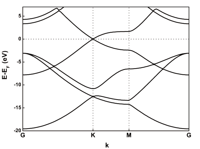
Fig. 1 Graphene band structure with VASP
You can improve the description of these states by increasing the
cutoff radii by hand in the PAO.Basis block in graphene.fdf.
However, even using orbitals with very long (and expensive) tails (up to 14 Bohrs),
the description of these bands is not accurate.
3. You can improve further the basis set using diffuse or ghosts orbitals. The file graphene.diffuse.fdf includes 3s and 3p orbitals with very long tails. These are enough to lower the energy of the \(\sigma^*\) states below 5eV. Alternatively, the file graphene.ghosts.fdf includes a layer of ghost orbitals (C-like) slightly above and below the graphene plane. By doing this we are able to describe electronic states that extend farther away from the atomic layer into the vacuum, at the cost of including a significant number of orbitals in the basis. You can compare your results with Fig. 2.
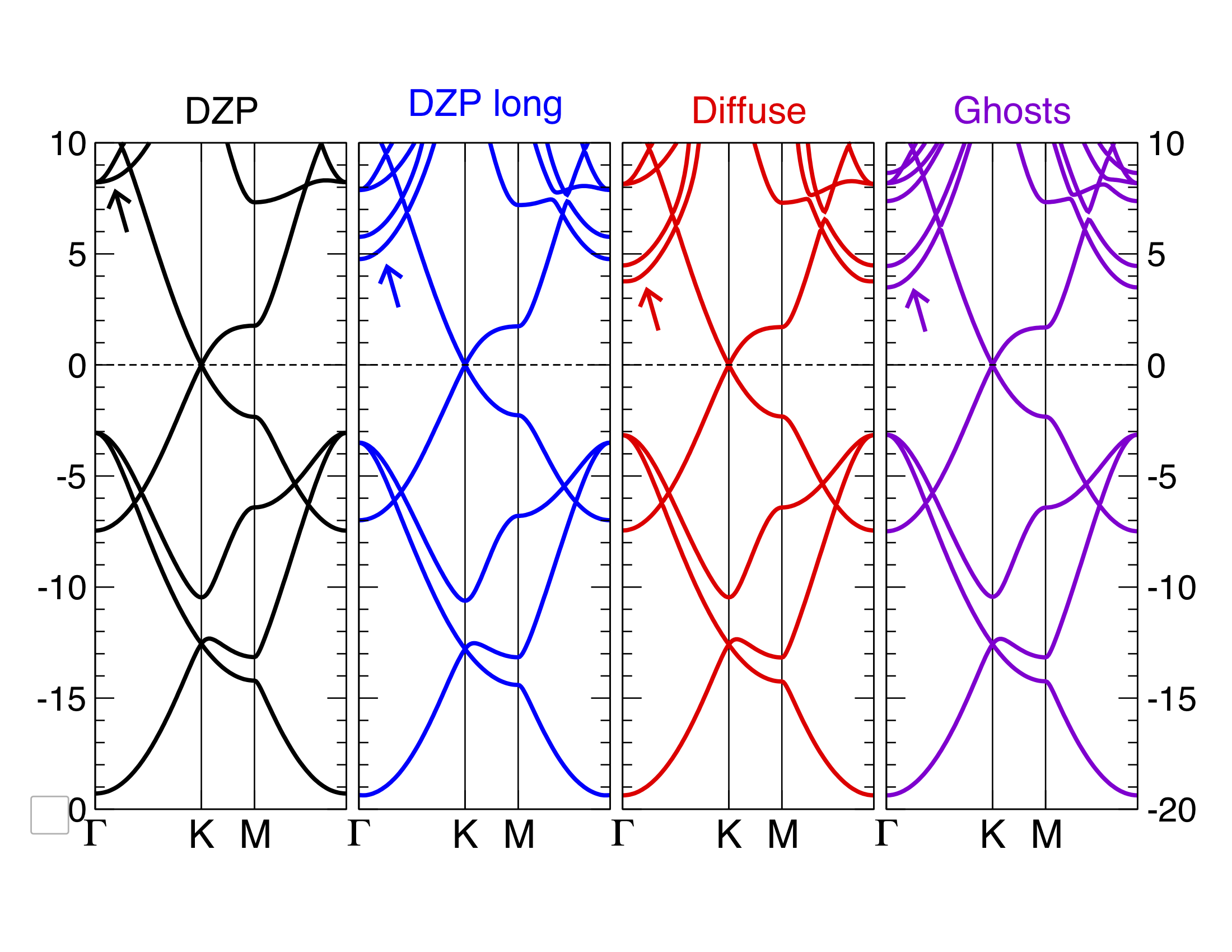
Fig. 2 Graphene bands with Siesta with various basis sets
You can try different types of basis also for the ghost orbitals and check the results.
The file GC.psf is a copy of C.psf, and is used to generate the basis of the ghost atom,
which must be defined in the ChemicalSpecies block (with a
negative Z; see the manual for details). You can use other type
of chemical species to define the ghosts.