The self-consistent-field cycle

Have you set up the local environment?

If not, do that now before proceeding.

In this exercise we will look more closely at the scf cycle (Fig. 6) and how to monitor its convergence

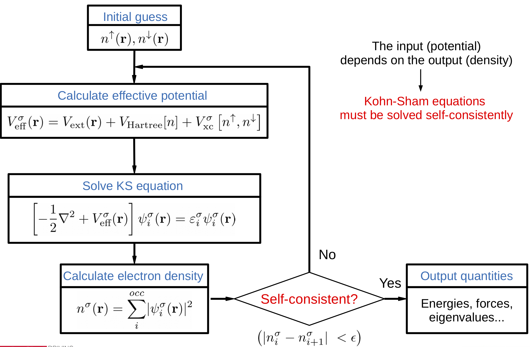
Fig. 6 Flow diagram of the scf cycle

Whether a calculation reaches self-consistency in a moderate number of steps depends strongly on the mixing strategy used. The available mixing options should be carefully tested for a given calculation type. This search for optimal parameters can repay itself handsomely by potentially saving many self-consistency steps in production runs.

In this tutorial we will see a brief summary of the options related to self-consistency, and will practice with them.

Note

Here we use the modern forms of the options. You might find legacy options in fdf files. They are still valid but are deprecated. Consult the manual for more information.

Siesta can mix either the density matrix (DM) or the hamiltonian (H), according to the flag:

SCF.mix  { density | hamiltonian }

The default is to mix the Hamiltonian, which typically provides better results.

It can be illustrative to look at a sketch of the code flow to understand the interplay between the DM and H, depending on the mixing options:

if ( mixH ) then

 call compute_DM( iscf )
 call compute_max_diff(Dold, Dscf, dDmax)

 call setup_hamiltonian( iscf )
 call compute_max_diff(Hold, H, dHmax)

else

 call setup_hamiltonian( iscf )
 call compute_max_diff(Hold, H, dHmax)

 call compute_DM( iscf )
 call compute_max_diff(Dold, Dscf, dDmax)

end if

(appropriate mixing here)

Note

Beyond the two main mixing methods, there are other experimental techniques that we will not discuss in this tutorial

There are two main ways in which the SCF condition can be monitored in SIESTA:

• By looking at the maximum absolute difference dDmax between the matrix elements of the new (“out”) and old (“in”) density matrices. The tolerance for this change is set by SCF.DM.Tolerance. The default is 10-4, which is a rather good value, valid for most uses, except when high accuracy is needed in special settings (some phonon calculations, or simulations with spin-orbit interaction).

• By looking at the maximum absolute difference dHmax between the matrix elements of the hamiltonian. The actual meaning of dHmax depends on whether DM or H mixing is in effect: if mixing the DM, dHmax refers to the change in H(in) with respect to the previous step; if mixing H, dHmax refers to H(out)-H(in) in the current step. The tolerance for this change is set by SCF.H.Tolerance. The default is 10-3 eV.

By default, both criteria are enabled and have to be satisfied for the cycle to converge. To turn off any of them, one can use one of the options:

SCF.DM.Converge F
SCF.H.Converge  F

The options to control the mixing are quite varied, and the manual should be studied to gain a full understanding. Here we will cover the more basic options.

The first is the method of mixing, controlled by SCF.Mixer.Method:

scf-mixer-method { linear | Pulay  | Broyden }

with linear mixing being the default. In this case, the mixing is controlled by SCF.Mixer.Weight (formerly DM.MixingWeight), which is 0.25 by default. This means that the program keeps 70% of the original DM or H, and adds to it 25% of the new one.

The Pulay and Broyden methods are more sophisticated: they keep a history of previous DMs or Hs (as many as indicated by the SCF.Mixer.History flag, which defaults to 2.

A simple example

In directory CH4 there is a ch4.fdf file very similar to the one in the first-contact tutorial, but with the mixing options modernized (and a DZP basis set).

Run the example with the provided parameters. Yoy will see that the program stops with an error regarding lack of scf convergence: it has not reached convergence in the allowed 10 scf iterations (set by the MaX-scf-iterations parameter. Before trying anything else you might want to increase the allowed number of iterations.

Play with the SCF.Mixer.Weight parameter to see if you can accelerate the convergence. Also, check the differences when mixing the DM or H.

You have probably noticed that using large values (close to 1), reaching convergence becomes extremely difficult or even impossible. However, if you use a large value, but now set the parameter scf-mixer-method to Pulay or Broyden, you will see that the SCF convergence is reached in a few iterations. Experiment with the values of SCF.Mixer.History and SCF.Mixer.Weight to see if you can find optimum values for a fast convergence.

A harder example

Directory Fe_cluster contains an example of a non-collinear spin calculation for a simple linear cluster with three Fe atoms.

The input file fe_cluster.fdf is set up to use linear mixing with a small mixing weight. Check how many iterations are needed for convergence.

Now experiment with other options, and see how much you can reduce the number of iterations.

When you are done, you might want to peruse the file scfmix.fdf, in which the new mixing technology in Siesta is exemplified (use of different strategies that can kick in under certain conditions, defined in blocks). You need to read the manual to follow the meaning of the options.

Note

See that we have commented out the DM-use-save-dm option. Otherwise, a new calculation in the same directory would re-use a (possibly converged, or half converged) DM file.

Note

If you have a hard-to-converge system, you might want to share it with the developers.