Sampling of the BZ with k-points

Author

Miguel Pruneda (ICN2) and Alberto Garcia (ICMAB-CSIC).

Have you set up the local environment?

If not, do that now before proceeding.

In this exercise we will explore the convergence with k-point sampling for a (semi)metalic system, and compare with an insulator. We have selected three carbon-structures that are particularly easy to converge in terms of basis and real-space mesh. You will work in the directories graphene, graphite, and diamond.

Hint

Enter the graphene directory

Here we will focus on a well-known 2D crystalline system: graphene

In the input file graphene.fdf a 4x4x1 grid is used:

%block kgrid_Monkhorst_Pack
4  0  0    0.5
0  4  0    0.5
0  0  1    0.0
%endblock kgrid_Monkhorst_Pack

As we will see, this is insufficient for a good description of graphene.

To plot the DOS we will use the utility program ‘Eig2DOS’. For the broadening for each state in eV (a value of the order of the default (0.2 eV) is usually reasonable, but if you want to reproduce the smooth V-shape close to graphene´s Dirac cone you will probably have to decrease that value). We can try:

Eig2DOS -f -s 0.1 -n 400 -m -12.0 -M 2.0 -k graphene.KP  graphene.EIG > dos

which will compute the DOS in the (12 eV ,2 eV) range around the Fermi level (-f option), using a grid of 400 points and a broadening of 0.1 eV.

The content of the ‘dos’ file can be plotted using gnuplot:

gnuplot
plot "dos" u 1:4 with lines

We get a set of spikes, with just some inkling that there might be a V-shaped feature near the Fermi level. Obviously the sampling is not good enough.

The file graphene.fdf will also produce a file graphene.bands containing the band structure along the several lines in the Brillouin zone (BZ) as specified using the block:

%block Bandlines
  1   0.5000000000   0.000000000   0.0000   M
 30   0.0000000000   0.000000000   0.0000   \Gamma
 45   0.3333333333   0.333333333   0.0000   K
 30   0.5000000000   0.500000000   0.0000   M
%endblock BandLines

To plot the band structure we use the utility program ‘gnubands’, taking advantage of some new features (type gnubands -h for a list of options):

gnubands -F -G -o bandstructure -E 10 -e -20 *.bands

that will shift the origin of energy to the Fermi level. With the above command we will get a window between -20 eV and 10 eV with respect to Ef. Also, a ‘bandstructure.gplot’ driver file is created automatically (which has extra information to place and label the ‘ticks’ for each symmetry point in the BZ). Now we plot:

gnuplot --persist -e "set grid" bandstructure.gplot

The position of the Dirac cone is highlighted by the gridline passing by the high-symmetry K point). It is obvious, however, by looking at the Ef gridline, that the Fermi level does not fall exactly at the Dirac cone, as it should (see Fig. 3).

Fig. 3 Graphene band structure

The position of the Fermi level in (semi)metals is very sensitive to the k-point mesh used. In this case, the 4x4x1 sampling originally set in the input file is clearly not appropriate. You can increase the Monkhorst-Pack parameters and check the convergence. Notice also that in graphene (and other hexagonal lattices) the K-point (1/3,1/3,0) is particularly relevant, and it is advisable that it is explicitly included in the discretization. In fact, in this case including the K-point makes all the difference, as can be seen by using this block:

%block kgrid_Monkhorst_Pack
 6  0  0    0.0
 0  6  0    0.0
 0  0  1    0.0
%endblock kgrid_Monkhorst_Pack

The Fermi level is now exactly at the vertex of the Dirac cone. But this is not really a consequence of having increased the density of k-points, but of including the K-point in the sampling (check the graphene.KP file, but note that the k-points are given in cartesian coordinates, not relative to the reciprocal basis vectors; can you see it?). In fact, if we use the block:

%block kgrid_Monkhorst_Pack
 3  0  0    0.0
 0  3  0    0.0
 0  0  1    0.0
%endblock kgrid_Monkhorst_Pack

leading to a much coarser sampling, we still get the Fermi level correctly aligned. The presence of the K point in the sampling set pins the Fermi level at the Dirac cone.

It is also instructive to see the behavior of the DOS when the k-point sampling gets more dense. For coarse samplings, it does not look at all like the “free-electron-like” curve we see in textbooks. This is due to the very simple method used to construct the DOS (just broadening a collection of discrete energy levels). You probably have to increase the mesh beyond 60x60x1 to have good plots for the DOS.

Note

You do not need to run again a full scf cycle to get the DOS with more k-points. You could re-use the converged density-matrix to shorten the cycle (option DM.use-save-dm). There is an alternative route that does not use the .EIG file, but the computation of the partial density of states. Just include the blocks:

%block ProjectedDensityOfStates
  EF -20.00  10.00  0.100  500  eV
%endblock ProjectedDensityOfStates

%block PDOS.kgrid_Monkhorst_Pack
 60  0  0    0.0
 0  60  0    0.0
 0   0  1    0.0
%endblock PDOS.kgrid_Monkhorst_Pack

and the program will compute the pDOS (and the DOS) in a finer grid. The DOS is in graphene.DOS, which can be plotted as:

gnuplot> plot "graphene.DOS" u 1:2 with lines

to get a figure similar to Fig. 4. (Note that the scf sampling was set to 6x6x1, as above). The pDOS information might be useful also.

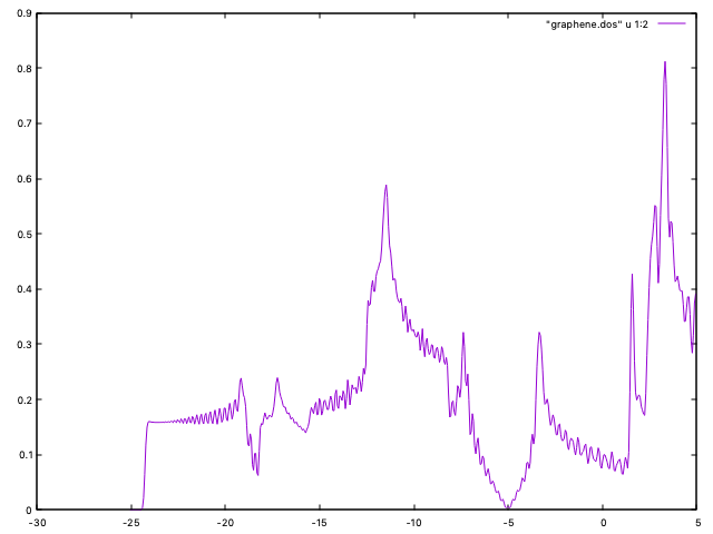
Fig. 4 Graphene DOS (60x60x1 k-sampling)

Hint

Enter the graphite directory

Graphite is the 3D version of graphene. It is a semimetal, and similar caveats than graphene apply. Now, however, the k-point sampling along the three spatial directions must be considered.

The input “graphite.fdf” includes the bandlines required to plot the bands. Notice that there is a flat band right at the Fermi level (compare with Fig. 5). Check the convergence of the Fermi level, and the DOS as a function of the k-sampling.

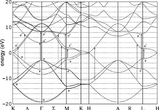
Fig. 5 Graphite bands

Hint

Enter the diamond directory

Finally, another 3D example is diamond. It has the same fcc structure as silicon, and the high-symmetry K points are included in the input file “diamond.fdf”. Unlike graphene and graphite, diamond is non-metallic, and the k-point convergence is easier. Plot bands, and DOS and check the results.