Atomic Populations¶

As seen in the theoretical background section, the equation for the total number of electrons can be re-arranged by partitioning the orbital index \(\mu\) into different subsets for different atoms:

\[N = \sum_I { \sum_{\mu\in I} { \sum_{\nu} { \sum_i { f_i c^i_{\mu}c^i_{\nu} S_{\mu\nu}}}}}\]

where I labels the different atoms. It is tempting to think of

\[q_I = \sum_{\mu\in I} { \sum_{\nu} { \sum_i { f_i c^i_{\mu}c^i_{\nu} S_{\mu\nu}}}}\]

as the “contribution of atom I” to the total charge of the system. These are the “Mulliken populations”.

However, the assignment of charge to “atoms” is an ill-defined problem in DFT (we really have an “electron soup” that has found its optimal arrangement). Different schemes exist, each with their own advantages and limitations.

Mulliken populations¶

The Mulliken populations are the most straightforward application of the partitioning above. They are printed by SIESTA if any of the following options is used in the fdf file (see the manual for more details):

# Old-style   (allowed values 0,1,3,4)
WriteMullikenPop 1

# New style:
Charge.Mulliken.Format 1   # Print Mulliken populations
Charge.Mulliken end        # Print at the end of the run

We can run SIESTA calculations for a water molecule with both DZP and SZ basis sets and compare the Mulliken populations.

Hint

Enter the H2O_populations directory

For example, for the water molecule with a DZP basis, we might get:

Mulliken Atomic Populations:
Atom #   charge [q] valence [e]  Species
   1     0.096949    5.903051  O
   2    -0.048475    1.048475  H
   3    -0.048475    1.048475  H

This seems to show that the oxygen atom has lost charge, and the hydrogen atoms have gained electrons, which is contrary to what one would expect on the basis of the relative electronegativities of H and O.

The problem is that Mulliken charges are explicitly sensitive to the basis set choice. Consider the following “gedanken experiment”: a complete basis set for a molecule could be set up in principle by placing a large set of functions on a single atom. In the Mulliken scheme, all the electrons would then be assigned to this atom. The method thus has no complete basis set limit.

In fact, if we use a SZ basis, we might get:

Mulliken Atomic Populations:
Atom #   charge [q] valence [e]  Species
     1    -0.674980    6.674980  O
     2     0.337490    0.662510  H
     3     0.337490    0.662510  H

which is closer to what one expects, despite using a “worse” basis set!

Hirshfeld and Voronoi populations¶

To address the limitations of Mulliken populations, SIESTA implements alternative schemes:

Hirshfeld populations:

Hirshfeld charges are a widely used method in quantum chemistry to assign partial atomic charges in molecules based on the electron density distribution. The fundamental idea is to partition the total electron density of a molecule, \(\rho(\mathbf{r})\), into atomic contributions using reference densities from neutral atoms.

The Hirshfeld method, sometimes termed the “stockholder” approach, defines a weight function for each atom A:

\[w_A(\mathbf{r}) = \frac{\rho_A^0(\mathbf{r})}{\sum_B \rho_B^0(\mathbf{r})}\]

Here, \(\rho_A^0(\mathbf{r})\) is the electron density of the isolated neutral atom A, located at the position it occupies in the molecule. The denominator sums over all atoms in the molecule. This weight function describes the spatial proportion of atom A at position \(\mathbf{r}\) compared to all other atoms.

Using this weight, the Hirshfeld atomic electron density for atom A is given by:

\[\rho_A(\mathbf{r}) = w_A(\mathbf{r}) \cdot \rho(\mathbf{r})\]

The Hirshfeld charge \(q_A\) on atom A is then calculated as:

\[q_A = Z_A - \int \rho_A(\mathbf{r}) d\mathbf{r}\]

where \(Z_A\) is the (pseudo) atomic number of atom A.

Voronoi populations:

The Voronoi polyhedron around an atom is the set of points that are closer to that atom than to any other. It is a 3D generalization of the Voronoi diagram in 2D. The Voronoi partial charge associated to an atom is simply the integrated density in the Voronoi polyhedron.

The computation of these atomic populations is requested with the options:

# Old style
WriteHirshfeldPop T
WriteVoronoiPop T

# New style
Charge.Hirshfeld end
Charge.Voronoi end

For the water molecule example above, these charges come out to be:

Hirshfeld Atomic Populations:
Atom #   charge [q] valence [e]  Species
     1    -0.253805    6.253805  O
     2     0.126903    0.873097  H
     3     0.126903    0.873097  H

Voronoi Atomic Populations:
Atom #   charge [q] valence [e]  Species
     1    -0.199738    6.199738  O
     2     0.099871    0.900129  H
     3     0.099868    0.900132  H

You can verify that these charges are indeed much less sensitive to the details of the basis set.

Plotting the charge density¶

In this section we will obtain a graphical representation of the charge transfer from H to O, using the grid information that Siesta keeps and optionally outputs to files.

Take a look at the last lines of the `h2o.fdf file (same for sz.fdf):

# Output files with charge densities

save-rho T
save-delta-rho T

With these options Siesta produces the files h2o.RHO and h2o.DRHO which contain, respectively, the valence charge distribution and the deformation density. They are Fortran binary files with the values of the appropriate 3D arrays on the points of the grid. We can convert them to a format that can be used by standard visualization tools by means of the grid-to-cube conversion tool g2c_ng (see more background in this how-to):

g2c_ng -s h2o.STRUCT_OUT -g h2o.RHO
mv Grid.cube RHO.cube

g2c_ng -s h2o.STRUCT_OUT -g h2o.DRHO
mv Grid.cube DRHO.cube

The g2c_ng program produces files in the .cube format. The renaming is needed because the file name is a generic “Grid.cube”.

Now we can use Vesta (among others) to load and display the content of the files. If we visualize the total charge density originating from the RHO file, we will see something like this:

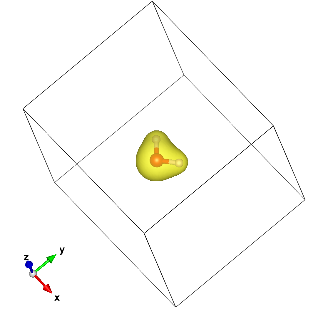
which is a rather boring blob. If we process the DRHO information (which is the difference between the final converged charge density and the density built as a superposition of atomic charges) we get instead:

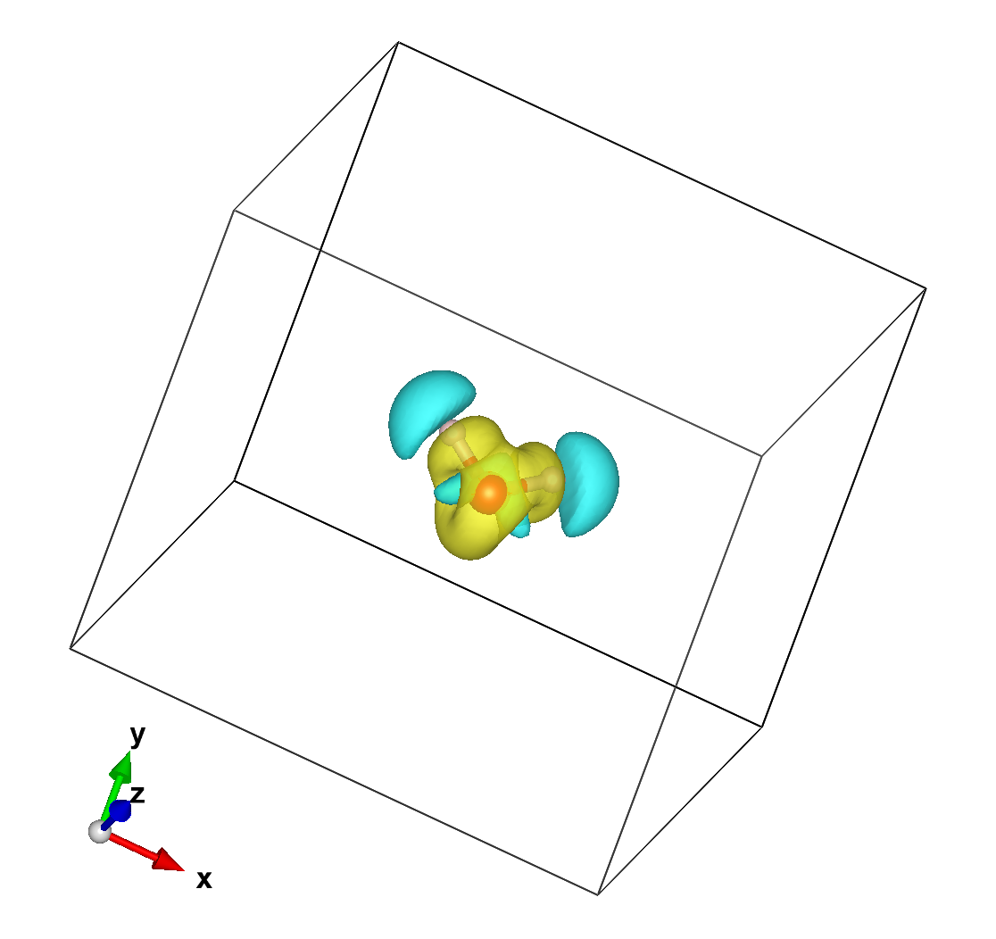
in which it is apparent that H has lost some charge and the neighborhood of O gained it.

Note

We can also use the rho2xsf tools to produce XSF files appropriate for the XCrysDen tool. See this how-to).

Oxidation states vs. DFT atomic populations¶

Hint

Enter the MgO directory

Magnesium Oxide is a rather ionic compound. The formal oxidation states for O and Mg are, respectively, -2 and +2. In a naive picture, Mg has lost its two valence electrons and O gained them. When one looks at the populations computed within DFT, however, the net losses or gains of charge by the atoms come out to be much smaller:

Mulliken Atomic Populations:
Atom #   charge [q] valence [e]  Species
     1     1.102318    0.897682  Mg
     2    -1.102318    7.102318  O

Hirshfeld Atomic Populations:
Atom #   charge [q] valence [e]  Species
     1     0.236801    1.763199  Mg
     2    -0.236800    6.236800  O

Voronoi Atomic Populations:
Atom #   charge [q] valence [e]  Species
     1     0.310257    1.689743  Mg
     2    -0.310257    6.310257  O

The Voronoi and Hirshfeld estimations of charge transfer are particularly small in this case.

Oxidation states are book-keeping tools based on assigning electrons to atoms using formal rules, which assume complete electron transfer (ionic limit). They’re useful for balancing reactions and understanding chemistry, but they don’t represent actual charge distributions.

Even in “ionic” compounds, bonding has significant covalent character, and electrons are shared, not completely transferred. (Notice the relatively small, but non-zero, band dispersion, as seen in the tutorial on band-structure)

Let’s recall again that the assignment of charge to “atoms” is in any case an ill-defined problem. The real observable is the electron density distribution. Atomic populations can serve at most to explore qualitative trends.