Projected Density of States (pDOS)

Do you want to get all tutorial materials on your local machine?

You can get all files and set up your local environment. Do that now before proceeding.

In our chain of equations in the background section we encoutered:

\[g_{\mu} (\varepsilon) = \sum_i { \sum_{\nu} { c_{i\mu}c_{i\nu} S_{\mu\nu} \delta(\varepsilon - \varepsilon_i) } }\]

which is the projected density of states (pDOS) over orbital \(\mu\). Note that when the basis is not orthogonal, the sum over \(\nu\) and the overlap factor are needed.

There are several utilities that can be used to process the projected DOS.

Hint

Enter the directory MgO

Projected DOS from a .PDOS or .PDOS.xml file

When a Projected-Density-of-States block is used in Siesta, such as:

%block Projected-density-of-states
-26.00 4.00 0.200 500 eV
%endblock Projected-density-of-states

Siesta will compute a full decomposition of the DOS over all orbitals, in the energy range provided (above: -26.00 to 4.00 eV), using a given broadening (0.2 eV above), and a given number of energy points in the range (500 in the above example). The output is placed, for historical reasons, in two files: SystemLabel.PDOS and SystemLabel.PDOS.xml. Both contain the same (XML) data, but the first one is formatted so that the data items appear in separate lines. The second is more compact. We have kept the original .PDOS file since it can be processed by the fmpdos program by Andrei Postnikov, which does not really parse the XML, and depends on the special format.

The program pdosxml uses an XML parser to process either file, and is therefore more robust. However, it currently has a drawback: the specification of which orbitals to take into account for the projection of the DOS is done in the code, so the program must be recompiled for each use. It is thus not very convenient in practice.

Both fmpdos and `pdosxml are installed when Siesta is built.

The shortcomings of pdosxml and fmpdos can be avoided by using a new python-based utility pdos-select, which offers a fully flexible orbital specification syntax and a host of other features. Some examples:

# Select all oxygen orbitals
pdos-select h2o.PDOS --select "species == 'O'" > oxygen_dos.dat

# Multiple selections (OR logic)
pdos-select input.PDOS --select "species == 'O'" --select "species == 'H'"

# Complex query
pdos-select input.PDOS --select "atom_index in range(1, 6) and l in [0, 1]"

# List all orbitals without processing
pdos-select input.PDOS --list-orbitals

# Export as CSV
pdos-select input.PDOS --select "l == 0" --format csv -o output.csv

# Get help on selection syntax
pdos-select --help-selectors

Note

pdos-select is not yet included in the Siesta distribution. To install it, assuming you have a modern Python interpreter installed, just execute:

pip install --index-url https://gitlab.com/api/v4/projects/27621639/packages/pypi/simple pdos-tools

The package has no extra dependencies.

The PDOS file can also be processed by sisl.

Note that if a different energy range, smearing, or number of points is desired, a new Siesta run must be used. And since the PDOS information is computed internally from the coefficients of the wave functions, the program needs the Hamiltonian, which cannot currently be read from a file. So even if a converged density-matrix file is used to restart the calculation, some substantial computing is still involved to get the new projected DOS data.

One can specify a denser BZ sampling for the PDOS calculation by using a special block:

%block PDOS.kgrid_Monkhorst_Pack
 8  0  0  0.5
 0  8  0  0.5
 0  0  8  0.5
%endblock PDOS.kgrid_Monkhorst_Pack

Projected DOS from wavefunction information

An alternative way to process the projected DOS is to use explicitly the equation for \(g_{\mu}(\varepsilon)\) at the top, which involves the overlap matrix and the wavefunctions associated to a full sampling of the BZ. These can be output to file by Siesta if the option:

COOP.write T

is used. The name of the option is related to the framework for the analysis of the crystal-overlap populations (COOP/COHP), which includes the processing of the pDOS as a by-product.

This framework allows the interactive control of all the parameters (energy range, broadening, orbitals involved, etc), at the expense of having potentially large wavefunction files around.

When SIESTA runs with the above option in the fdf file, it will generate a file MgO.fullBZ.WFSX. To process the pDOS information one can use the mprop utility:

mprop [option] dos

which, among other things, implements the equation for \(g_{\mu}(\varepsilon)\) at the top, using the selection of orbitals on which to project specified in the file dos.mpr.

Note

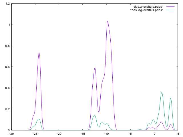
In this example, dos.mpr specifies two projections: on the Mg orbitals, and on the O orbitals:

MgO
DOS
Mg-orbitals
Mg
O-orbitals
O

The first line is the system label (MgO), while the second indicates the type of property we are calculating (DOS in this case). The following lines go by pairs, and they include 1) the name for the output files and 2) the orbital selection. So in this case we get the PDOS for the Mg orbitals and store it in the dos.Mg-orbitals.pdos files, and then we get the PDOS for the O orbitals and store it in the dos.O-orbitals.pdos files.

You could add more lines to plot PDOS over different orbital sets if you want, or be more specific in your orbital selection. For example:

• projection over the pz orbitals of O can be obtained by using O_pz as the orbital selection string.

• Mg_2s will project over all 2s orbitals in Mg.

If you want further information on how to define orbitals, try with mprop -h.

You can select the range of energy (eV), or the band range for which you plot the DOS, the number of energy points, and the smearing (Gaussian) used:

mprop -n 500 -b 1  -B 5 -s 0.4 dos

This generates files dos.*label*.pdos with the projected DOS. In those files, the first column is the energy (in eV), the following columns contain the different spin components, and the last column has the spin-sum over the orbitals. The total DOS (considering all orbitals) is also saved into dos.ados. You can easily plot the projections with gnuplot:

gnuplot
gnuplot> plot "dos.O-orbitals.pdos" u 1:4 w l, "dos.Mg-orbitals.pdos" u 1:4 w l

or use the provided pdos.gplot script:

gnuplot -persist pdos.gplot

Note that this scheme for the computation and analysis of the pDOS is more flexible than the one based on the direct production of .PDOS files by Siesta. It allows to change the smearing, number of points, and energy range. On the other hand, it requires to store a potentially large file with wavefunctions.