Band Structure

Do you want to get all tutorial materials on your local machine?

You can get all files and set up your local environment. Do that now before proceeding.

We have been using this expression for the expansion of the wave-functions in localized orbitals:

\[|\Psi_i> = \sum_{\mu} { c^i_{\mu} |\mu>}\]

This is fine for molecules, but for extended (periodic) systems (e.g. crystals, two-dimensional slabs, one-dimensional nano-structures) we use Bloch’s theorem and employ an extra label for the wave-functions, the k-point. Using explicitly the real-space form:

\[\psi_{n\mathbf{k}}(\mathbf{r}) = \sum_{\mu, \mathbf{R}} c_{\mu,n\mathbf{k}}\, e^{i\mathbf{k}\cdot(\mathbf{R} + \mathbf{d}_{\mu})}\, \phi_{\mu}(\mathbf{r} - \mathbf{R} - \mathbf{d}_{\mu})\]

This equation shows also the SIESTA convention of using the actual position of the orbital in the unit cell (\(\mathbf{d}_{\mu}\)) in the phase factor.

The eigenvalues \(\epsilon_n({\mathbf{k}})\) are also labeled by k-point \({\bf k}\) and the band index \(n\). The set of k-points spans the so-called Brillouin Zone, which is essentially the Wigner–Seitz cell (or Voronoi polyhedron) in reciprocal space, formed by drawing perpendicular bisectors between the origin and all other reciprocal lattice points. See the Wikipedia article on Brillouin Zone for more details.

Let’s now learn how to visualize this band structure.

Hint

Enter the MgO directory

The input file MgO.fdf requests SIESTA to print the information of the band structure along high-symmetry lines in the Brillouin zone (BZ):

BandLinesScale     ReciprocalLatticeVectors

%block BandLines                  # These are comments
1  0.000  0.000  0.000  \Gamma   # Begin at Gamma
25  0.500  0.000  0.500     X     # 25 points from Gamma to X
10  0.500  0.250  0.750     W     # 10 points from X to W
15  0.500  0.500  0.500     L     # 15 points from W to L
20  0.000  0.000  0.000  \Gamma   # 20 points from L to Gamma
25  0.375  0.375  0.750     K     # 25 points from Gamma to K
25  0.625  0.250  0.625     U     # 25 points from K to U
%endblock BandLines

Let’s understand these few lines:

• The BandLinesScale entry specifies the scale of the k-vectors given in the BandLines block. The possible options are “ReciprocalLatticeVectors” and “pi/a” (deprecated).

• Each line of the BandLines block represents the end-point of a segment to be spanned in the reciprocal space.

Note

To learn more about the special high-symmetry points and lines of the BZ for other systems, you can visit the Bilbao Crystallographic Server. As of this writing, this link is down due to maintenance.

Note

An alternative tool to generate high-symmetry points in the BZ is Seekpath, which can also be used online at the Materials Cloud. The online version can read, among others, POSCAR files, which are similar to Siesta’s STRUCT_OUT files.

Information about the bands is stored in the file MgO.bands. To plot the band structure you can use the utility program gnubands:

gnubands -h  # To see the options
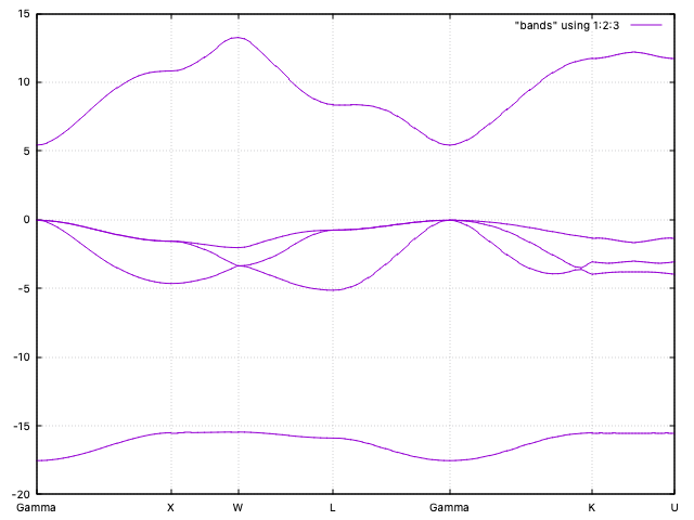
gnubands -G -o bands -F -b 1 -B 5 MgO.bands

With the above command we are requesting a plot of the first 5 bands (4 of them are occupied (why?)), shifting the energy values so that the Fermi level is at 0 (the top of the valence band in this case). In addition, we request labels por the high-symmetry points at the ticks. The command will generate automatically a gnuplot script in the file bands.gplot, which can be used to obtain the plot:

gnuplot -persist -e "set grid" bands.gplot

The grid setting is optional, but it helps to align the band features. The bands are quite flat, as it fits a mostly ionic compound (why?).