DFT+U calculations¶

Author: Daniel Sanchez Portal (2010), based on the file provided by P. Aguado and J. Junquera

We will be working with manganese oxide (MnO). This compound has a NaCl structure, that is, an FCC lattice with a basis of two atoms. However, the ground state of MnO corresponds to a ferromagnetic alignment of the Mn atoms within the (111) planes and the antiferromagnetic alignment of those planes, as shown in Fig. 8.

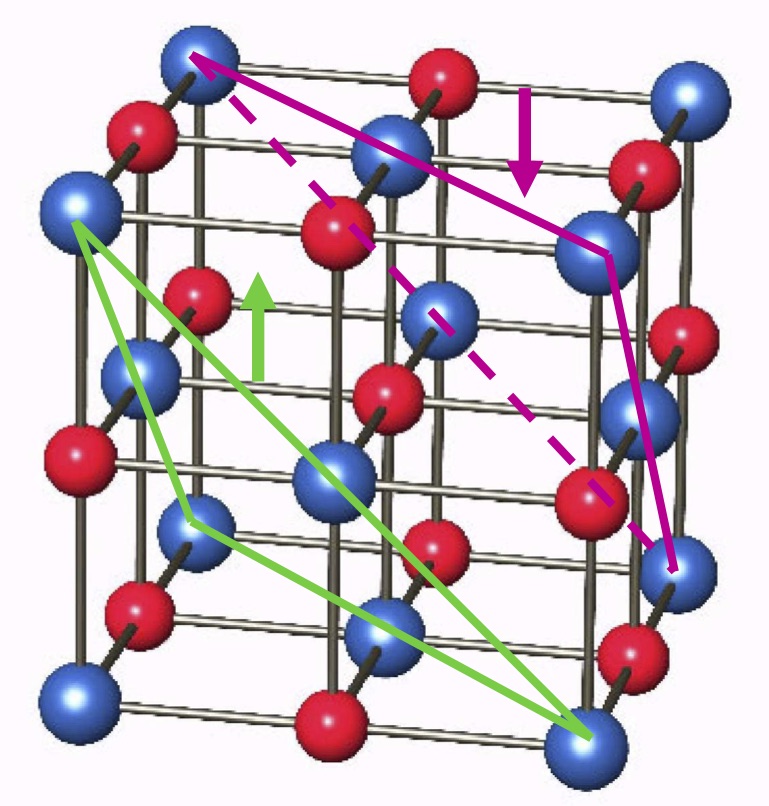
Fig. 8 AF2 structure of MnO¶

Look at the input file, MnO.fdf, and study the different variables.

Pay special attention to the variables we are focusing on, those related to the LDA+U approximation, the band structure calculation and the Projected Density of States (PDOS) calculation. Check their meaning in the User’s Guide:

%block LDAU.proj
Mn   1               # number of shells of projectors
n=3    2             #  n, l
<U_value>  0.000     # U(eV), J(eV)
  0.000    0.000     # rc, \omega (if zero default values are taken)
%endblock LDAU.proj

%block BandLines
1     2.000 0.000  0.000 X
40    0.000 0.0000 0.000 Gamma
15    0.500 0.5000 0.500 Z
%endblock BandLines

%block ProjectedDensityOfStates
     -25.00  10.00  0.200  600 eV
%endblock ProjectedDensityOfStates

Also, check the meaning of

WriteMullikenPop 1         # Orbital Mulliken Populations 

We are considering the antiferromagnetic AF2 arrangement of MnO. You can check that we are starting from an antiferromagnetic alignment looking at the block:

%block DM.InitSpin
1  1.0
2 -1.0
3  0.0
4  0.0
%endblock DM.InitSpin

Running SIESTA and changing parameters¶

Change the value of the U parameter for the GGA+U calculation appears in the input file (MnO.fdf) in the block:

%block LDAU.proj
Mn   1               # number of shells of projectors
n=3    2             #  n, l
<U_value>  0.000     # U(eV), J(eV)
0.000    0.000     # rc, \omega (if zero default values are taken)
%endblock LDAU.proj

We suggest to use first the value U=0.0 and then increase the value of U in steps of 1 eV up to, for example, U = 5 eV.

Let’s start with U=0.0:

$ siesta < MnO.fdf > out.U=0.0

You should keep the following information from each run: the output file, the MnO.bands file, and the MnO.PDOS file.

Thus, after each run you should change the names of these files so they are not overwritten, i.e. for example

$ mv MnO.bands MnO.U=1.bands

Magnetic alignment in the SCF solution¶

You can edit now the output files from any of the previous runs and check the value of the spin moment. In fact, the antiferromagnetic alignment remains and the total moment is zero.

You can check that the total moment is zero in the output:

siesta: Total spin polarization (Qup-Qdown) =    0.000000

However, although the total spin moment is zero the local moments in the Mn atoms are different from zero. The local moments can be obtained by analyzing the Mulliken populations in the output:

mulliken: Atomic and Orbital Populations:

mulliken: Spin UP

Species: Mn
Atom  Qatom  Qorb
             4s      4s      4Ppy    4Ppz    4Ppx    3dxy    3dyz    3dz2
             3dxz    3dx2-y2 3dxy    3dyz    3dz2    3dxz    3dx2-y2
 1  5.554   0.006   0.241   0.143   0.143   0.143   0.989   0.989   0.958
            0.989   0.958  -0.015  -0.015   0.021  -0.015   0.021
 2  0.846  -0.078   0.264   0.119   0.119   0.119   0.038   0.038   0.111
            0.038   0.111  -0.007  -0.007  -0.007  -0.007  -0.007

 etc...

Note

Which is the spin moment in each Mn atom?

Yes, each Mn atom in the cell has a spin moment of ~4.7 Bohr magnetons. While the moment in atom 1 points in the up direction, it points in the down direction for atom 2.

You can also check that the Oxygen atoms are not polarized.

Plot the band structure¶

Run the program gnubands to produce to plot the band structure from the raw data produced by SIESTA.

gnubands < MnO.U=2.bands > bandas.MnO.U=2

(The source code of gnubands.x, gnubands.f can be found in the /Util directory of the standard SIESTA distribution.) [ORG: Modify this]

Recall that you can check the position of the Fermi energy in the head of the “.bands” files.

You can now plot the bands using gnuplot:

$ gnuplot
gnuplot> plot "bandas.MnO.U=0" w l, "bandas.MnO.U=3" w l

so you can compare the bands with different values of U.

To produce a postscript file with one of the previous figures:

gnuplot> plot "bandas.MnO.U=0" w l, "bandas.MnO.U=3" w l
gnuplot> set terminal postscript
gnuplot> set output "MnO.bands.ps"
gnuplot> replot
gnuplot> quit

To generate a pdf file from the previous postscript:
```
$ ps2pdf MnO.bands.ps
```

Is the size of the gap increasing? Are all the bands equally modified/shifted?

PDOS plots¶

Since the +U correction is only applied to the 3d shell of Mn, only the position of those states with a significant contribution from the Mn 3d orbitals are modified.

To check this it is interesting to plot the projected density of states projected on the different orbitals. For this we will use the utility pdosxml. This utility can usually be found in the /Util directory of the standard SIESTA distribution. For more information, please see this how-to.

Assuming you have versions of pdosxml to extract the pDOS for the Mn 3d orbitals on atoms 1 and 2, and for the oxygen atom, do:

pdosxml_Mn3d_atom1 < MnO.U=3.PDOS > Mn3d_atom1
pdosxml_Mn3d_atom2 < MnO.U=3.PDOS > Mn3d_atom2
pdosxml_O < MnO.U=3.PDOS > O

As the name clearly indicates, the file Mn3d_atom1 will contain the PDOS on the 3d orbitals of Mn atom 1 and so forth. You can also use the fmpdos tool mentioned in the above how-to document.

You can plot these PDOS as a function of U using gnuplot and check that those states with strong Oxygen contribution do not change significantly as we increase U.