Nudged Elastic Band (NEB) Calculations¶

Author: Arsalan Akhtar (ICN2)

Note

For more details and images, you can refer to this slide presentation.

In these two exercises you will learn how to calculate the barriers in materials using the so-called Nudged Elastic Band approach (NEB).

Note

These exercises use the Lua scripting engine inside Siesta, and need the FLOS library to be installed. If you have not done so, please follow the instructions here.

The NEB method [ref] is based on the refinement of earlier “Chain-of-states” method. The aim of a chain-of-states calculation is to define the minimum energy path (MEP) between two local minima. The MEP is found by constructing a set of images of the system (a chain-of-states, on an “elastic band”) between the initial and final configuration. An optimization via minimization of the effective forces acting on the states in the elastic band will bring the images to the MEP.

The basic procedure of the NEB technique with siesta is as follows:

Initialize the first set of images, based on the linear interpolation between the initial and final images.
Relax your initial and final images
Re-interpolate between initial and final images to generate new images.
Run the NEB algorithm using LUA script.

Note

Usually the initial and final images should first be relaxed before interpolation. which means the to endpoint states are in valley of PES.

Note

The examples are NOT completely optimized and are just practical examples for this tutorial. For real calculations, one needs to properly optimize all the parameters such as kpoints, mesh, basis sets, etc.

Example-1: Water Molecule Rotations¶

In this example we going to calculate the barriers required to rotate one water molecule in the neighbourhood of another water molecule as shown in Fig. 16.

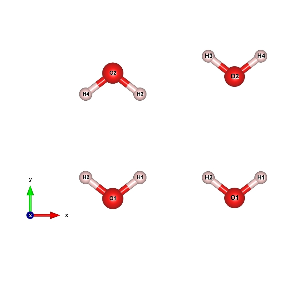
Fig. 16 initial (left) final (right) image/structure of Water¶

Go to directory neb-example-1 , you will find there two SIESTA input files called input.fdf and parameters.fdf, pseudopotential files for H and O, and six interpolated image_* files for the rotating water molecule. We will later show how we generated those images. There will be also a lua script file named neb.lua, which contains the top-level logic for the NEB algorithm. Finally, the plot-neb.py script will plot the NEB results. If you open the parameters.fdf you will see:

MD.TypeOfRun LUA
Lua.Script neb.lua

Which tells Siesta to use the provided lua script to perform a specific task (now a NEB calculation). Now open input.fdf , you see we are using a constraint block to fix some atom positions and allow only two H atoms to move!:

%block Geometry.Constraints
  atom [1 -- 4]
%endblock Geometry.Constraints

You can run siesta as usual:

siesta < input.fdf | tee output.out

Hint

With Intel Core-i7 (3.8 GHz) 8 cores it will cost ~10 mins!

Note

DM.History.Depth 0 Flag should be set to be Zero which allow to reuse the DM but in “neb.lua” script we have not provided this feature.

While running siesta you could use following commands to retrive the NEB forces:

grep NEB: <NAME OF YOUR OUTPUT FILE>

You should see somthing like this:

NEB: max F on image 1 =    0.85434, climbing = false
NEB: max F on image 2 =    0.84249, climbing = false
NEB: max F on image 3 =    0.79173, climbing = true
NEB: max F on image 4 =    0.77845, climbing = false
NEB: max F on image 5 =    0.79005, climbing = false

Once the calculation finished and converged to desired NEB force threshold you will find something like:

NEB step
NEB: max F on image 1 =    0.01032, climbing = false
NEB: max F on image 2 =    0.01780, climbing = false
NEB: max F on image 3 =    0.02324, climbing = true
NEB: max F on image 4 =    0.03045, climbing = false
NEB: max F on image 5 =    0.03684, climbing = false

LUA/NEB complete

Now we use the plot_neb.py script to plot the barrier profile:

python plot_neb.py

Note

If you open the plot_neb.py script there will be two parameters to check : Number_of_images & NAME_OF_NEB_RESULTS. The user should provide the correct info!

You should get a plot like Fig. 17.

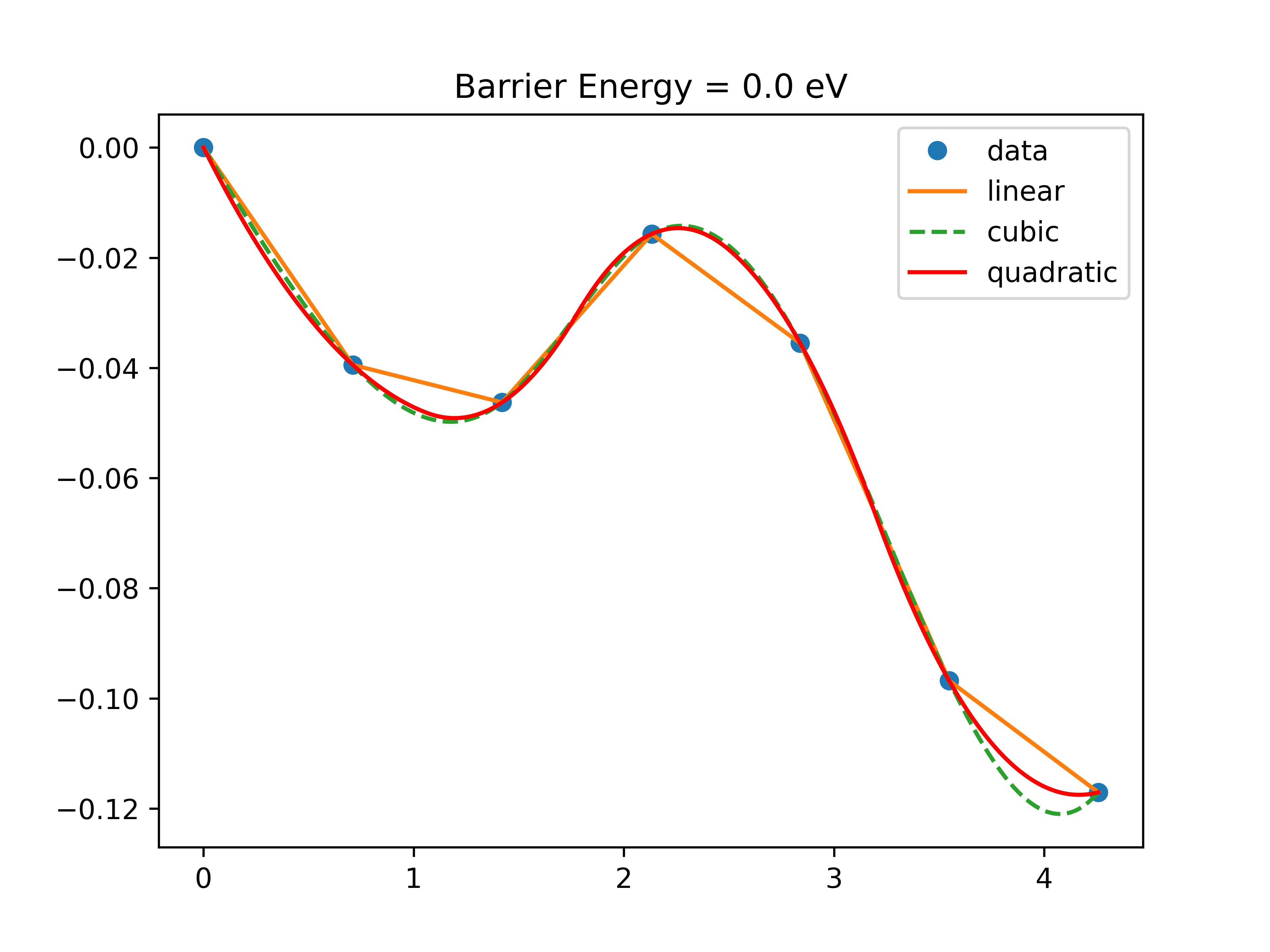
Fig. 17 Water rotation barrier¶

Digging more into the NEB LUA Script¶

To learn more about flos library we refer you to the flos documentation site, but for now we focus on two important things:

1. NEB parameters such as spring constant, number of images,label,...etc.
2. Optimizer of NEB

if you open neb.lua in first lines of script you will find:

-- The prefix of the files that contain the images
local image_label = "image_"

-- Total number of images (excluding initial[0] and final[n_images+1])
local images, n_images = {}, 5

-- The default output label of the DM files
local label = "NEB"

you have to be careful with image_label, n_images and label. The first one is the prefix for the name of image files and the second one is the number of images that you generated excluding initial and final image. Finally the label of file which the NEB info will be dumped. to change the k spring constant you have to look for

-- Now we have all images...
local NEB = flos.NEB(images)

and change it to desired values like this (here we change it to 1):

-- Now we have all images...
local NEB = flos.NEB(images,{k=1})

regarding the optimizers have to look for

-- Setup each image relaxation method (note it is prepared for several
-- relaxation methods per-image)
local relax = {}
for i = 1, NEB.n_images do
   relax[i] = flos.FIRE{direction="global", correct="global"}
end

and modify it to the optimizers of your choice like (here we choose CG):

-- Setup each image relaxation method (note it is prepared for several
-- relaxation methods per-image)
local relax = {}
for i = 1, NEB.n_images do
   --relax[i] = flos.FIRE{direction="global", correct="global"}
  relax[i] = flos.CG{beta='PR',restart='Powell', line=flos.Line{optimizer = flos.LBFGS{H0 = 1. / 25.} } }
end

Generating images with SISL¶

For sure you are now familiar with sisl. If not you could refer to this tutorial. Here we use sisl to rotate the H around O.

import sisl

# Read initial geometry
init = sisl.Geometry.read('input.fdf')

# Create images (also initial and final [0, 180])
for i, ang in enumerate([0, 30, 60, 90, 120, 150, 180]):
    # Rotate around atom 3 (Oxygen), and only rotate atoms
    #  [4, 5] (rotating 3 is a no-op)
    print("Rotating {} angle H with 4,5 index ".format(str(ang)))
    new = init.rotate(ang,v=[0,0,1], origo=3, atoms=[4, 5], only='xyz')
    new.write('image_{}.xyz'.format(i))
new.write('initial.fdf')
new.write('final.fdf')
print("Image Generated!")

Example-2 Hydrogen Hopping on Graphene¶

Now we are going to study the hopping of hydrogen atoms in graphene.

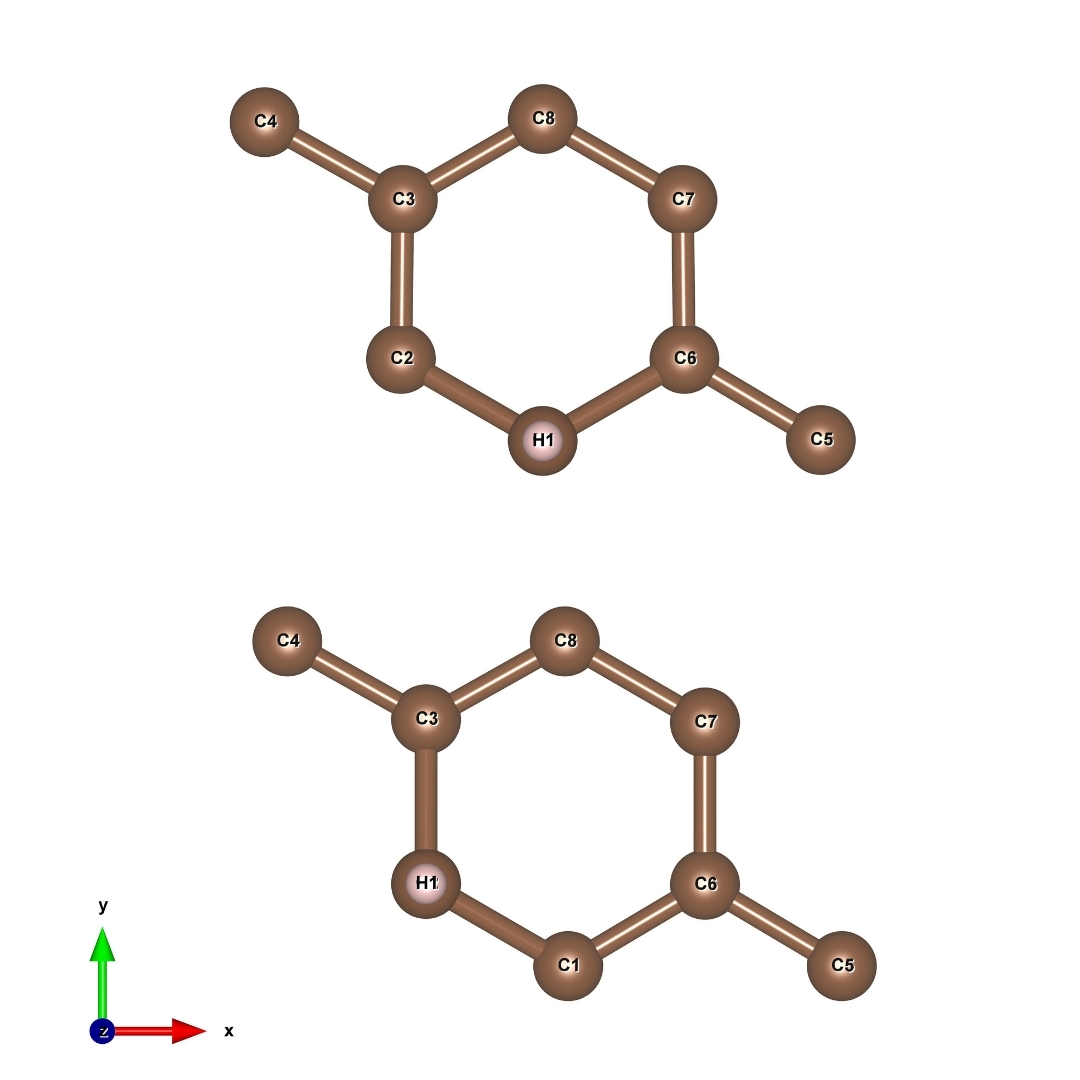
Fig. 18 initial (up) final (bottom) image/structure of Graphene-H¶

Hint

Go now to directory neb-example-2

You will find there two directories initial and final which contain Siesta input files called initial.fdf , final.fdf and parameters.fdf and pseudopotentials for C and H (now in psml type).

Now, to start, you have to relax the initial and final structures. Then you will be able to generate intermediate images using the script provided (check the next section). After generating the images you have to copy those images into neb folder.

Now you are ready to go and run the calculation for NEB but first look in parameters.fdf to check that this flags are set:

MD.TypeOfRun LUA
Lua.Script neb.lua

Which tell Siesta to use the provided lua script to perform a specific task (now a NEB calculation).

Note

Here if you look into neb.lua (line 75+) you will find that we are now using CG optimizer for this NEB. the flos library contains different types of optimizers. You could also use lbfgs Optimizer.

-- Setup each image relaxation method (note it is prepared for several
-- relaxation methods per-image)
local relax = {}
for i = 1, NEB.n_images do
   --relax[i] = flos.FIRE{direction="global", correct="global"}
  relax[i] = flos.CG{beta='PR',restart='Powell', line=flos.Line{optimizer = flos.LBFGS{H0 = 1. / 25.} } }
end

Hint

This example might require more time ~ 90 mins with Intel Core-i7 (3.8 GHz) 8 cores

Generating images with ASE¶

Here we use the Atomic Simulation Environment (ASE) to generate the images and then pass it to sisl to write it in Siesta fdf format if we want.

import sisl , ase
from ase.neb import NEB

number_of_images = 7            # Try for different images!
interpolation_method = 'idpp'   # Try 'li' for linear interpolation

#Try For Unrelaxed Structures Uncomment #
#-------------------------------------------------------------------------------
#FDF_initial = sisl.get_sile("<PATH TO FDF FILE *.fdf OF INITIAL STRUCTURE>")
#FDF_final = sisl.get_sile("<PATH TO FDF FILE *.fdf OF FINAL STRUCTURE")
#-------------------------------------------------------------------------------

# If You Relaxed
FDF_initial = sisl.get_sile("<PATH TO XV FILE *.XV OF INITIAL STRUCTURE>")
FDF_final = sisl.get_sile("<PATH TO XV FILE *.XV OF FINAL STRUCTURE")

#===============================================================================

Geometry_initial = FDF_initial.read_geometry()
Geometry_final = FDF_final.read_geometry()
ASE_Geometry_initial = Geometry_initial.toASE()
ASE_Geometry_final = Geometry_final.toASE()

images = [ASE_Geometry_initial]
print ("Copying ASE For NEB Image  0")
for i in range(number_of_images):
    print ("Copying ASE For NEB Image ",i+1)
    images.append(ASE_Geometry_initial.copy())
images.append(ASE_Geometry_final)
images.append(ASE_Geometry_final)
print ("Copying ASE For NEB Image ",i+2)
neb = NEB(images)
neb.interpolate(interpolation_method)

Now we use plot_neb.py script to plot the barrier.

python plot_neb.py

you should get a plot like this:

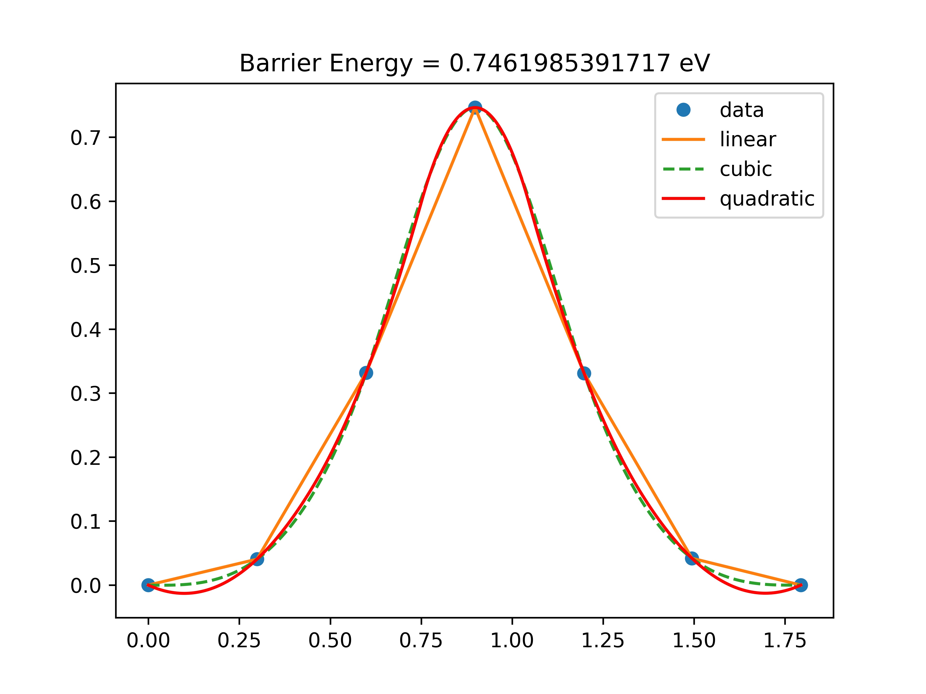
Fig. 19 Hydrogen hopping barrier¶

Further points of study¶

If you manage to run/get results now try:

Check the number of images required to have a good barrier resolution.
Check the number of iterations required for converging NEB with `li` and `idpp` interpolation methods
Could you converge the graphene example with FIRE optimizer? If
   not, what could you try?
Check the LFBGS optimizer for water case. Is it faster?
How does the Spring constant influence the computed barriers?