Spin-Orbit coupling
- Author
Ramón Cuadrado (University of Southampton)
The main goal of this tutorial is to cover the basic notions to perform calculations using the Spin-Orbit-Coupling (SOC) implementation in Siesta.
Note
It is mandatory to take into account this when SOC is included in the calculation:
converge the k–points sampling
converge the mesh cutoff
converge the density matrix with a tolerance below 10^-5
use relativistic pseudopotentials (PPs) and use the non–linear core corrections when the PPs are built.
All the information regarding the basis set and all the parameters used in a common SIESTA calculation are valid for the SO.
In the next two examples the above mentioned parameters (mesh cutoff, etc) are not converged because we want to speed up the calculations to show an initial (and dirty) results, but remember, for a real calculation those values have to be converged.
An additional advice: remember to read the SOC section in the main Siesta manual!
Calculation of the magnetic anisotropy of Pt2.
Hint
Please move to directory Example-1
Note
The original fdf for this example can be found in example_1z.fdf.original. We have made some changes (can you see them?) to speed the calculation while maintaining reasonable quality results.
Given the example_1z.fdf file and the pseudopotential of Pt atom, Pt_pt2_SOC.psf, calculate the total selfconsistent energy Etot for three highly symmetric orientations of the initial magnetization, namely, X, Y and Z, keeping fixed the physical dimer (the (x,y,z) coordinates of each atom).
Each calculation has to be initialized modifying the DM.InitSpin, updating the orientation of
each atomic magnetization. As a result one has to have three different
energy values for each (θ,ϕ) pair.
Remember to rename each one of the .fdf files (and the SystemLabel flag inside) for each magnetic orientation, and do not use the density matrix obtained in other orientations as it has to be calculated for each specific magnetic configuration from scratch.
Note
You can also try to change the orientation of the dimer (say put it along the Z or Y axes) and compute again the energy values associated to different spin orientations and compare the results. Some of the total energies (which?) have to be the same.
Calculation of the magnetic anisotropy of FePt bulk
Hint
Please move to directory Example-2
Note
The original fdf for this example can be found in example_2z.fdf.original. We have made some changes (can you see them?) to speed the calculation while maintaining reasonable quality results.
You will find the example_2z.fdf file and the PPs of Fe and Pt: Fe_fept_SOC.psf
and Pt_fept_SOC.psf (note that the pseudo for Pt is different from
that in the first example). Each calculation has to be initialized modifying
the DM.InitSpin block, as above, updating the orientation of each atomic
magnetization. As a result one has to have three different energy values
for each (θ,ϕ) pair.
A) Obtain the Etot for three highly symmetric orientations of the initial magnetization, namely, X, Y and Z, keeping fixed the atoms in their unit cell. Again do not use the same density matrix for same calculations. Allow SIESTA to calculate it from scratch.
B) Create a magnetization curve changing the angles at intervals of 20 degrees from the Z-axis inital orientation, to finalize along the X axis. Plot the resulting energy as a function of the varied angle. One can check the magnetic moments, charge, etc.
These set of calculations will take lot of time to be performed completely, so you can try a few steps and see how the total energy evolves.
Note
If you do plot the magnetization curve, you might see that it has a minimum at around 60 degrees, which does not make too much sense, and it is quite shallow. In this case we went too far in the simplification of the parameters to gain speed. In particular, removing the polarization orbitals has a very significant effect. At the cost of a noticeably longer simulation time, you can restore those orbitals by using the block:
%Block PAO.Basis
Fe_fept_SOC   2
n=4   0   2  P
0.0   0.0
n=3   2   2
0.0   0.0
Pt_fept_SOC   2
n=6     0       2  P
0.00000     0.00000
n=5     2       2
0.00000     0.00000
%EndBlock PAO.Basis
You should now get a curve similar to that in Fig. 7:
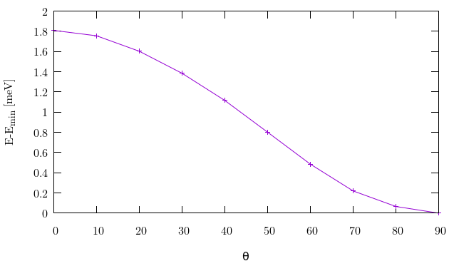
Fig. 7 Magnetization curve from Z to the X axis
Spin Projected Density of States (collinear case)
Hint
Please move to directory Example-3
Note
The original fdf for this example can be found in example_3.fdf.original. We have made some changes (can you see them?) to speed the calculation while maintaining reasonable quality results.
In example_3.fdf we have included the block:
%block ProjectedDensityOfStates
  -10.00  5.00  0.02  1000  eV
%endblock ProjectedDensityOfStates
After Siesta runs we will have a file called example_3.DOS and example_3.PDOS, containing the information on the DOS and PDOS, respectively.
( You can modify the parameters in the block as needed, and run Siesta after the modification. You might want to use a pre-converged .DM file.)
Plot the example_3.DOS using gnuplot. In doing this you will see the total DOS of the system. If you want to see the atomic resolved DOS (PDOS on atoms, for example), you have to extract from the PDOS file the parts that represent the Fe/Pt DOS.
Note
The PDOS file can be processed as discussed in this how-to.
You can plot the PDOS↑, PDOS↓for each specie or the total DOS (the sum of the relevant columns). It is worth noting that in general, for the transition metals the most relevant orbitals will be the d ones.
Projected Density of States (fully relativistic case)
Hint
Please move to directory Example-4
Note
The original fdf for this example can be found in example_4z.fdf.original. We have made some changes (can you see them?) to speed the calculation while maintaining reasonable quality results.
When the Spin–Orbit coupling is included in the calculation the PDOS and DOS files will have four columns corresponding to PDOS↑, PDOS↓, and Re PDOS↑↓ and Im PDOS↑↓, such that the integral of Re PDOS↑↓ up to EF will give the magnetization along X axis, Mx, and the integral of Im PDOS↑↓ up to EF , My
(For a noncollinear calculation without SOC, the files will have the same structure as those for SOC and hence four columns will be written in the DOS/PDOS output files.)
Run Siesta using example_4z.fdf as input, and plot the total DOS.
You can use the self-consistent density matrix (label.DM) to calculate the DOS/PDOS. In this case the calculation is quite quick and the calculation of the DM from scratch is fast but in other cases it would be better to have the DM file and not calculate it again. So if you want copy it from the calculations in the directory Example-2 and use it!
Note
More advanced work: You can play with the DOS/pDOS analysis programs to choose other PDOS curves.