Calculation of optical properties
Note
For background, please see the slides for a lecture on the subject in a previous Siesta school.
- Author
Daniel Sánchez Portal (CFM-CSIC, San Sebastian), Alberto Garcia (ICMAB-CSIC)
In this exercise you will calculate the optical properties (imaginary and real part of the dielectric function and other derived quantities) using Siesta for two different structures of boron nitride: c-BN and h-BN.
Note
The formalism in this exercise is based on first-order perturbation theory. There is an alternative way to compute the optical response based on Time-Dependent Density-Functional Theory (TD-DFT), which is covered in another tutorial.
We use an automatic DZP basis set of moderately localized orbitals. The basic idea is that you become familiar with the different switches in the input that allow performing such a calculation.
The way to tell SIESTA that you want to perform a calculation of optical properties is to set:
OpticalCalculation T # or .true.
SIESTA will then compute the imaginary part of the dielectric function \(\epsilon_2(\omega)\) and will dump it in the file System_label.EPSIMG, which can be later post-processed to obtain optical quantities.
Hint
The pseudopotentials needed are in files B.psf and N.psf in the top directory of working files for this tutorial. You will need to copy them to the appropriate subdirectories (or use links) before running Siesta. For example, inside c-BN.10x10x10.0.3:
ln -sf ../B.psf ./B.psf
ln -sf ../N.psf ./N.psf
(Check first, as the links might already be there for you in some installations)
K-sampling and broadening
For a solid you need to specified a k-space grid to sample the different optical (i.e., vertical) transitions along the Brillouin zone. You do that using the block:
%block Optical.Mesh
    10 10 10
%endblock Optical.Mesh
A related parameter is Optical.Broaden, which sets the artificial
broadening applied to every transition so the calculated quantities
will appear as a smooth function and not as a collection of
spikes.
The effect of different k-space meshes nxnxn and broadenings a is analyzed for c-BN using the different input files inside the directories with names of the form c-BN.nxnxn.a.
A reasonably good sampling and smooth curve seems to be obtained with a 10x10x10 mesh and a broadening of 0.3 eV.
Hint
While doing these tests you will repeat several times the same calculation to converge the electronic structure with a scf cycle. Therefore, it is very convenient that you copy the density matrix (file c-BN.DM) from the first converged calculation to restart the new calculations:
Once you have done a first calculation, and from the working directory, type:
cp c-BN.DM ..
to copy the DM to the parent directory. Then, in subsequent calculations, from the particular working directory, type:
cp ../c-BN.DM .
Note that a copy operation, and not a link is used, as the DM file is over-written by the calculation.
Number of bands
Notice that all the previous calculations have been performed using
only 10 bands. This means that we have calculated the optical
transition matrix elements only between the 10 lowest bands (out of
the 26 that we have for BN using a DZP basis). The number of bands
used in the calculation can be controlled using the parameter
Optical.NumberOfBands. If it does not appear or is set
to a very large number, then all the bands will be used in the
calculation. Although not obvious in the present example, this will
considerably increase the time required for the computation in many
cases while it does not substantially improve the description of the
optical properties at lower energies.
It is important to take into account that the transitions for very large energies will not be reliable in most cases due to the limitations of the basis set: a large basis set, with large angular momenta, is necessary to describe electronic states at high energies. However, with Siesta and a DZP basis set you will be typically able to obtain a reasonable description of the optical properties of most materials below, say, ~10 eV, and up to ~20 eV using more complete basis set that incorporate more excited orbitals (particularly, higher values of l).
The input in the directory c-BN.10x10x10.0.3.allbands uses all the bands. We will see that the differences between both calculations (10 bands versus 26 bands) is only noticeable for energies higher than 25 eV, and the difference is tiny. We can thus continue restricting our calculations to the 10 lowest bands. It has to be noticed, however, that the deviations from the fulfilment of the f-sum rule will be larger the smaller the number of bands. This is important for the accuracy of the Kramers-Kroning transform necessary to obtain the real part of the dielectric function and, from this, other related quantities like the refraction index or the reflectance.
Scissor operator
Standard DFT methods usually lead to an underestimation of the band gap. This effect can be removed from the optical properties by applying an ad-hoc shift of the unoccupied bands as specified by ‘Optical.Scissor’. This approach is usually known as the ‘scissor operator’. Fig. 15 provides an illustration for the case of the Silicon band structure.
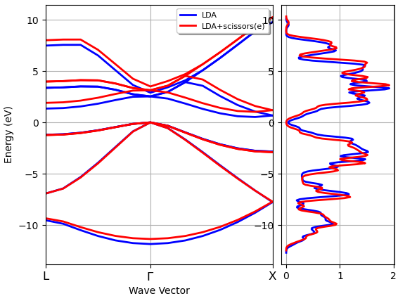
Fig. 15 Band structure of Si with scissors operator (taken from Abinit documentation)
You can check its effect running the calculation in ‘c-BN.10x10x10.0.3.scissor’, which defines:
Optical.Scissor 3.000 eV
Light polarization
Up to this point, all the calculations have been performed for linearly polarized light with a well defined direction of the electric field. This is defined using the input options:
Optical.PolarizationType polarized
%block Optical.Vector
   1.000 0.000 0.000
%endblock Optical.Vector
The possible choices for Optical.PolarizationType are polarized, unpolarized and polycrystal. For the ‘unpolarized’ option the propagation direction of light is defined, but the different directions of the electric field within the perpendicular plane are averaged. Using the ‘polycrystal’ option all possible directions are averaged.
Since c-BN is a cubic material, all these options should give the same result. You can check this running the calculation in ‘c-BN.10x10x10.0.3.polycrystal’ and comparing with previous results.
Non-isotropic materials
Finally, hexagonal boron nitride (h-BN) is not isotropic. Since it is a layered material, its optical properties parallel to the BN planes and perpendicular to the BN plane will be substantially different. Run the calculations in ‘h-BN.inplane’ and ‘h-BN.outplane’ to check this.
Note that in the h-BN.inplane case, rather than specifying a definite polarization direction within the plane, we request an unpolarized calculation with a light-propagation vector along z to average the in-plane response.
How to process the EPSIMG file
To compute the optical properties of a solid from the file
Systemlabel.EPSIMG that contains the imaginary part of the
dielectric function, we can use the programs optical_input and
optical`, which reside in the Util/Optical directory of the
Siesta distribution.
The first program creates the input file for the second. To do so, you just need to type:
optical_input < Systemlabel.EPSIMG
The program will create the file ‘e2.dat’ if there is not spin polarization, or the files ‘e2.dat.spin1’ and ‘e2.dat.spin2’ for the spin polarized case, and will output some text.
If the f-sum rule is not fulfilled by an amount larger than certain percentage specified in the program via the parameter THRESHOLD, the imaginary part of the dielectric function will be appended by a tail of the form
where C and p are determined to ensure continuity and to enforce the f-sum rule. This should increase the quality of the quantities determined via the Kramers-Kroning relations, however it is not very sophisticated and in certain cases it can create pathological problems. Anyway, it can be easily deactivated by setting the parameter THRESHOLD to zero (for this, use the sources to the program in the analysis directory in the working files for this tutorial).
The program optical (executed with no arguments or redirections)
reads the ‘e2.dat’ file containing the (possibly enhanced, as above)
imaginary part of the dieletric function, and creates the file
‘e1.interband.out’ that contains the real part of the dieletric
function, and ‘e2.interband.out’, which is the imaginary part
calculated back from the data in ‘e1.interband.out’. This serves as a
cross check of the quality of the Kramers-Kroning transformation.
For metals it is also necessary to include a Drude term (associated to intraband transitions) of the form
where \(\omega_p^2\) (the square of the plasma frequency) has been calculated by Siesta and appears at the beginning of the file Systemlabel.EPSIMG, and \(\gamma\) is an empirical parameter, the inverse of the relaxation time.
Also, it creates the files:
‘epsilon_real.out’ containing the real part of the dielectric function
‘epsilon_img.out’ containing the imaginary part of the dielectric function
‘refrac_index.out’ containing the refraction index
‘absorp_index.out’ containing the extintion coefficient
‘absorp_coef.out’ containing the absorption coefficient in cm**-1
‘reflectance.out’ containing the reflectance
‘conductivity.out’ containing the optical conductivity in (ohm*m)**-1