Advanced topics in phonons

author

Andrei Postnikov (Univ. Lorraine)

Note

For background, see the excellent slide presentation for a lecture by Andrei Postnikov in a previous Siesta school.

Note

There is some extra material for this tutorial here.

Note

To fully appreciate the issues in this tutorial you need to have understood the concepts presented in the basic vibrations tutorial.

The supercell explosion

We are going to consider a monolayer of BN, with two atoms per unit cell. In directory Phonon_Q we have already generated a 5x5x1 supercell with fcbuild (see the basic vibrations tutorial), by specifying:

Supercell_1  2
Supercell_2  2
Supercell_3  0

The supercell contains 50 atoms, and we should do in principle 2x6=12 calculations displacing the two atoms in the unit cell in the positive and negative cartesian directions to compute the forces on all the atoms in the supercell. That is a lot of work, so we have prepared a FC file for the rest of the exercise.

You need to copy this pre-generated FC file: cp BN.FC_save BN.FC, and then run vibra: vibra < BN_vibra.fdf. You will get the BN.bands and BN.vectors files.

The BN.bands file holds the phonon dispersion information, that you can plot with:

gnubands -G -o bnq BN.bands
gnuplot --persist bnq.gplot

You will get something like

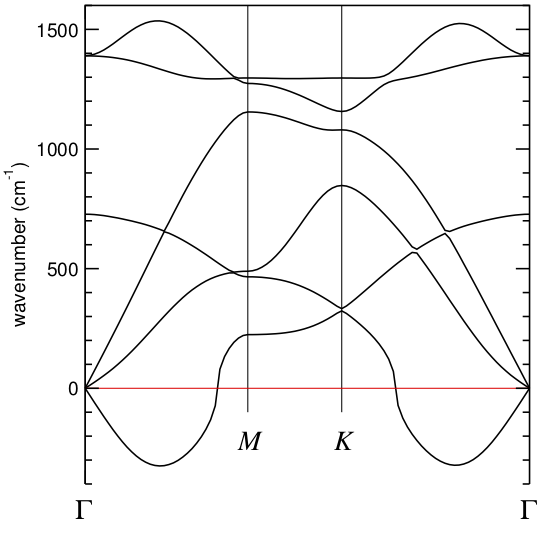
which looks quite bad in a neighborhood of Gamma.

Obviously, to improve on this we should increase the size of the supercell, maybe going to 7x7x1, 9x9x1, or even larger. The prospect is not pleasing.

But there is another way. Instead of generating a “brute force” supercell, we can generate a supercell that will describe correctly the dispersion along the high-symmetry directions that we care about. In this particular case, we can construct, following the indications in the slide presentation, a supercell that will exactly map the K and M points to Gamma. This is not the supercell for bookkeeping of the force-constants, but a new “unit cell” that serves our purposes.

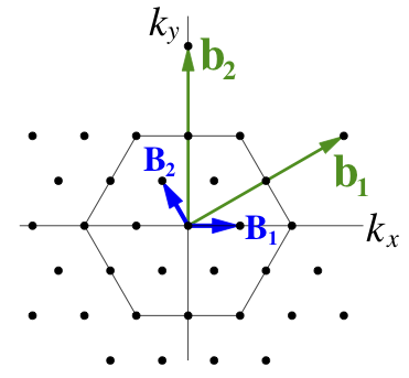
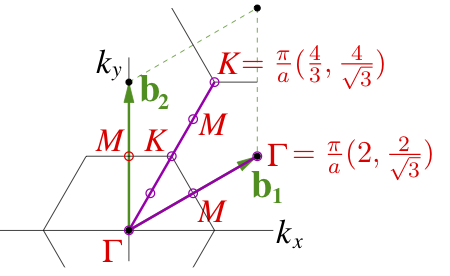
The process starts in the BZ, chosing new unit vectors to define a lattice that will include M and K:

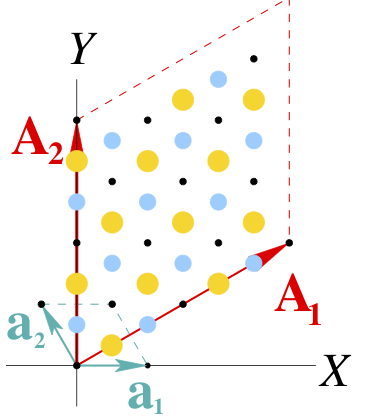
The reciprocal cell of this new unit cell is the real-space supercell we seek:

In directory Phonon_GMK we have the necessary files to compute the phonons at Gamma in this new “enlarged unit cell”. Now, with 24 atoms, we would need 24*6=144 calculations. It is a bit more CPU than the original case above (12 calculations for 50 atoms, each about 8 times more expensive than one for 24 atoms). Instead of running the calculations, you can use the provided FC file. (Copy the BN_save. files to use simply the prefix BN)

Run vibq0 and use the BN SystemLabel when asked. It will read the BN.FC and BN.XV files and produce .bands and .vectors files, just like vibra, but with a much simpler interface when only the Gamma point is handled.

In this case, the plotting is different because there is a single q-point:

gnubands -G -o gamma  BN.bands
gnuplot

gnuplot> plot "gamma" using 1:2 with points

and you will get a column of points marking the frequencies of the zone-center phonons in this enlarged unit cell. Not very useful compared to the original dispersion. All the modes are piled up at Gamma, and we need to unfold them.

Note

There are fundamental similarities between this problem and that of the unfolding of electronic bands covered in this tutorial, but the techniques are different.

Unfolding the Gamma “phonon structure” in the supercell

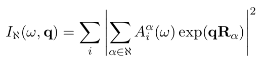
The character of these different modes can be revealed by projecting their eigenvectors onto waves with different Q-vector (see the lecture liked-to above):

The projection is done by the phdos program which is part of the lattice dynamics analysis package.

In order to probe projections onto different symmetric points of the BZ, the following coordinates of Q-points can be specified (in Cartesian coordinates and units of 1/Bohr, omitting the 2*pi factor). For A=2.495 Bohr:

M [0, 2*pi/(a*sqrt(30), 0] -> [0, 0.2314029, 0], or
M [pi/a, pi/(a*sqrt(3)), 0] -> [0.2004008, 0.1157014, 0];
K [2*pi/(3*a), 2*pi/(a*sqrt(3)), 0] -> [0.1336005, 0.2314029, 0];
K [4*pi/(3*a), 0, 0] -> [0.2672011, 0, 0]

according to the picture:

We have prepared the G.inp, K.inp, M.inp files to run the program. For example:

phdos < G.inp

mv BN.WSQ  BN.G.WSQ
mv BN.VSQ  BN.G.VSQ

will produce a .VSQ and a .WSQ file, which we rename for convenience and clarity. To plot the contents of the second one, which is more useful:

gnuplot
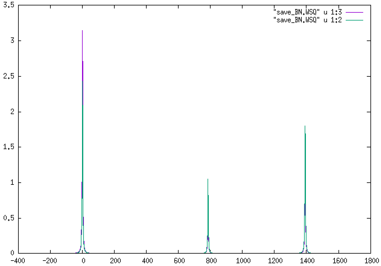
gnuplot> plot "BN.G.WSQ" u 1:3 w l
gnuplot> plot "BN.G.WSQ" u 1:2 w l

We will get sharp peaks at the positions of the “true” Gamma phonons (three acoustic modes with zero frequency, an intermediate one, and a degenerate optical mode), as in this figure:

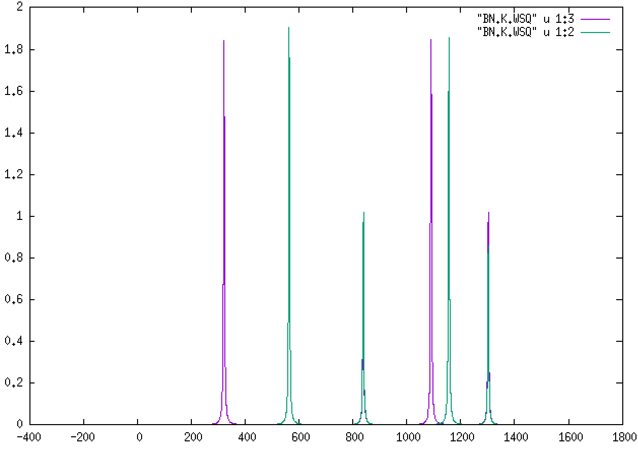
We can do the same for the K and M points. For K:

For M:

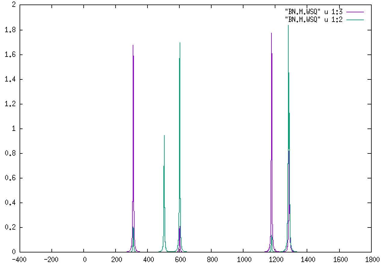
The two different colors correspond to the B and N atoms’ role in each mode. Being lighter, B will feature more prominently in the higher-frequency modes.

Can you check whether the phonons at K and M match the values in the general dispersion in the first section?

Can you think of which q-vectors to use with phdos to see whether we get better results in the lines Gamma-K and Gamma-M?

Note

One would be tempted to get a “dispersion” by selecting arbitrary q-vectors along a line and feeding them to phdos. However, it should be noted that we have really computed only 3N modes, where N is the number of atoms in the supercell. For some q’s we will get sharp peaks, but for others the signal will degrade and it would be difficult to make out “frequencies”.

Hint

The .VSQ files might be useful to get the frequencies of the peaks, as they have no broadening.

Note

There is an alternative method to compute the phonon dispersion at arbitrary q*s in the BZ, using only *unit cell calculations. It is based on Density-Functional Perturbation Theory. While convenient, this route removes half the fun of understanding supercells and folding issues.

LO-TO splitting and Born dynamical charges

Here is a picture of the phonon dispersion in hexagonal BN:

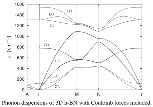
The LO-TO splittings at Gamma, in a 3D system, are caused by the effect of the electric field that the optical modes produce. There is an extra term in the force constants:

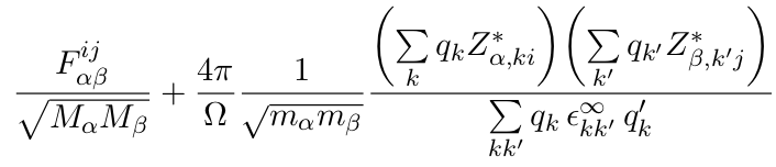
The second term is non-analytic, in the sense that it has different limiting values when q–>0 depending on the direction in which we approach it.

The Z’s in the above equation are the Born effective or dynamical charges, and can be computed as the derivative of the polarization in the crystal with respect to the atomic displacement, as shown in this tutorial, which you might enjoy following. In fact, the Born charges for hexagonal BN are explicitly calculated there, so you could go ahead and estimate roughly the size of the extra terms in the dynamical matrix for specific directions.

There is one extra ingredient: the \(\varepsilon_\infty\) in the non-analytic term is the clamped-ion dielectric constant, which can be computed using the methods outlined in the tutorial on optical properties.

We will not carry out any more specific calculations here, but it is worth noting the subtle links of the topic of phonons with other domains.

Also, it is apparent that to fully analyze a given system you might have to do several kinds of simulations: force-constants, Born charges, dielectric constant, etc. Ideally, you would set up an automated workflow that can help you manage everything. See the AiiDA framework tutorial for more information.

Note

Another use of the Born charges is in computing the infrared intensities of the modes. Only a few modes (those which involve changes in the polarization) would be infrared-active.

The vibra program can compute the infrared intensities if both the FC and the BC (for Born charges) files are available. See the Siesta and Vibra manuals for more information.