Examples of bonding analysis through COOP/COHP curves
Note
You can refer to this slide presentation for some extra material related to this tutorial.
COOP and COHP curves for a chain of N atoms
Hint
Enter directory N_chain
Here we will deal with this very simple system:
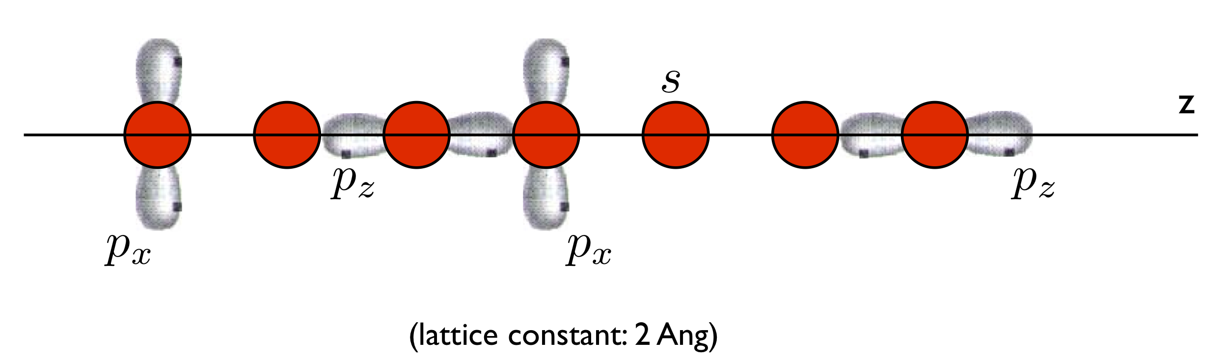
Explore the n_chain.fdf file to make sure you understand how the system is setup (in particular, how periodic boundary conditions are ued in this example), and run Siesta on it.
Note the ‘COOP.Write T’ line in the file. This forces the creation of the files n_chain.fullBZ.WFSX and n_chain.HSX, which contain wave-function and Hamiltonian and Overlap information, respectively.
These files can be processed by the mprop program (full documentation
available typing mprop -h) to obtain the DOS, PDOS, COOP, and COHP
curves for an arbitrary combination of orbitals.
Before using mprop, issue the following command to link the WFSX file to the name expected by the program:
ln -sf n_chain.fullBZ.WFSX n_chain.WFSX
Then type:
mprop pdos
to generate PDOS information (see file pdos.mpr). The curves can be plotted with the pdos.gplot script:
gnuplot --persist pdos.gplot
Now look at the n_coo.mpr file (which we have annotated here):
n_chain
COOP
N-N      --- name of the curve
N             -- first orbital kind (here: all on N)
1.95 2.05     -- distance range in Ang (to catch just nearest neighbors)
N             -- second orbital kind
N2s-N2px   : another curve
N_2s           : only 2s orbitals
1.95 2.05
N_2px          : only 2px orbitals on the second atom
N2px-N2px  : another curve
N_2px
1.95 2.05
N_2px
N2s-N2pz   : another curve
N_2s
1.95 2.05
N_2pz      : another curve
N2s-N2s
N_2s
1.95 2.05
N_2s
If we now type:
mprop n_coo
we will generate COOP and COHP curves for each of the sections highlighted. These display the energy-resolved bonding and antibonding character in the system. (Refer to the slide presentation linked-to above for extra graphical material.)
Spin instability in “non-magnetic Iron”
Hint
Enter directory Fe_spin_instability
This example is inspired by the discussion in the LOBSTER site. One can compute the electronic structure of a hypothetical phase of iron without spin polarization, i.e., non-magnetic. While it is obvious that the total energy of this system is higher than that of the true, spin-polarized ground state, one can look at the COOP/COHP curves to get a deeper view.
In directories Fe_magnetic and Fe_non_magnetic you can find .fdf files for the two cases.
Hint
Enter directory Fe_non_magnetic
Note how in the .fdf file we have deactivated the spin-polarization option.
You can now follow the same steps as detailed above for the first COOP/COHP analysis example:
siesta fe_cohp_nonmag.fdf | tee fe_cohp.nonmag.out
ln -sf fe_cohp_nonmag.fullBZ.WFSX fe_cohp_nonmag.WFSX
mprop fe_coo
to get the COOP/COHP curves and the total DOS. Note how in the fe_coo.mpr file we use the correct SystemLabel for this example:
fe_cohp_nonmag
COOP
Fe-Fe
Fe
2.0 3.0
Fe
We specify a spatial range of 2 to 3 ang for the orbital pairs, to get nearest-neighbor atoms, and in principle select all the orbitals in the Fe atom (but you might explore the contributions of particular pairs of orbitals, as in the example of the chain of N atoms).
You can plot the COHP curve with the command:
gnuplot --persist coo.gplot
You should get something similar to this:
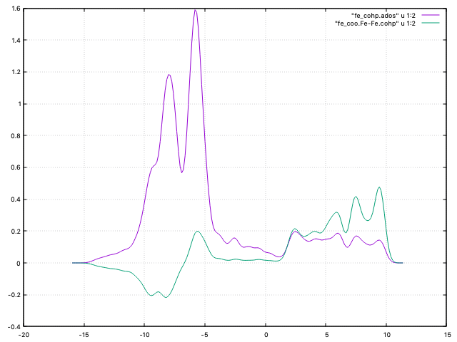
Fig. 9 DOS and COHP curve for non-magnetic Fe
The Fermi level for this system is approximately at -5.8 eV. We can see that there is a significant positive peak of the COHP curve at that energy, so there is a rather large non-bonding contribution when we consider the energies up to the Fermi level.
Hint
Enter directory Fe_magnetic
If we repeat the analysis for the “true” spin-polarized case (exercise for the reader!), we will obtain a lower total energy, and a COHP curve similar to this:
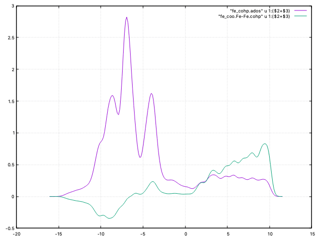
Fig. 10 DOS and COHP curve for magnetic Fe
which has a much smaller non-bonding contribution up to the Fermi level (-5.9 eV in this case). Note that we have combined in the coo.gplot script the up and down channels of the curves, for a better comparison with the non-magnetic case.
As discussed in the LOBSTER site, this is just one of a multitude of examples in which the COOP/COHP curves can shed light over bonding and stability issues.
References
Hoffmann, Roald. 1987. How Chemistry and Physics Meet in the Solid State., Angewandte Chemie International Edition in English 26 (9): 846–78.
R. Dronskowski, P. E. Blöchl, J. Phys. Chem. 1993, 97, 8617–8624 [COHP definition];
Sanchez-Portal, Daniel, Emilio Artacho, and Jose M Soler. 1995. “Projection of Plane-Wave Calculations into Atomic Orbitals.” Solid State Communications 95 (10): 685–90.
More LOBSTER references:
V. L. Deringer, A. L. Tchougréeff, R. Dronskowski, J. Phys. Chem. A 2011, 115, 5461–5466 [projected COHP definition];
S. Maintz, V. L. Deringer, A. L. Tchougréeff, R. Dronskowski, J. Comput. Chem. 2013, 34, 2557-2567 [The mathematical apparatus and the framework on which LOBSTER is built].
S. Maintz, V. L. Deringer, A. L. Tchougréeff, R. Dronskowski, J. Comput. Chem. 2016, 37, 1030-1035 [LOBSTER 2.0.0 and its nuts and bolts].