Spin texture
- author
Roberto Robles (CFM-CSIC) and Alberto Garcia (ICMAB-CSIC)
Notes on the Siesta implementation
Mathematically, the spin texture is simply a vector field: (non-collinear) spins in reciprocal space. In Siesta, the spin vector associated to a given spinor \(\Psi_{nk}\)
where \(\mathbf \sigma\) is a vector of Pauli matrices, can be computed using the coefficients of the spinors and the overlap matrix (appearing because of the space integral implied above).
The wave-function (spinor) coefficients are stored in a WFSX file, which can be created during a Siesta calculation in several ways:
Using the ‘BandPoints’ or ‘BandLines’ blocks (see manual), together with the option:
Wfs.Write.For.Bands T
Using the WaveFuncKpoints block to specify k-points and bands
Using the ‘COOP.Write T’ option: a wave-function set using the k-point sampling of the BZ used in the scf cycle will be written (see manual).
In general what one needs depends on the system. Many times simply having the spin texture along the directions of maximum symmetry, the same ones used to plot the band structure, is enough. In those cases BandLines serves perfectly. A regular sampling can be interesting when one does not know anything about the shape of the band and is interested in the texture of spin in the whole area of the Brillouin Zone. It would be the brute force option.
In cases with Dirac cones (graphene, topological insulators, etc), a radial sampling around the Dirac point (or in concentric circles with equispaced points) is usually what gives the best information. This is what we will use in the example below.
The spin_texture program can process the information and output,
for each \(n\bf k\) state selected, the spin vector.
The selection of states is on the basis of an eigenvalue interval (the whole range of energies in the file by default), or by band range.
Analysis of the spin-texture for a Bi2Se3 multilayer
Here we will use as an example a system composed of three quintuple layers of Bi2Se3.
The initial Siesta calculation uses the bi2se3_3ql.fdf file. Look at the options and you will see that, apart from converging the electronic structure, we request the band structure. This is useful to know what to analyze next. Other relevant pieces of information in the fdf file are:
SpinOrbit T
The block to initialize the spins to zero...
Upon executing the file with Siesta, we will get a bi2se3_3ql.bands file, that we can use to plot the band structure. Here it is useful to have an idea of what to plot, because there are many bands.
Hint
Before reading further, find out how many electrons there are in the system, and hence approximately how many bands are expected to be full (careful: this is a non-collinear spin calculation, and the bands are singly-occupied).
Something that is always useful is to employ the -F option of the
gnubands program to select a range of energies around the Fermi
level. In this case, we can look at the bands in a 1 eV window around
the Fermi level by:
gnubands -G -F -o around_ef -e -0.5 -E 0.5 bi2se3_3ql.bands
gnuplot --persist around_ef.gplot
You should get a picture similar to Fig. 11.
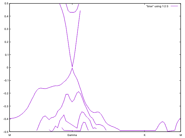
Fig. 11 Bands for Bi2Se3 multilayer near the Fermi level
We see clearly a Dirac cone.
We can plot the bands in a different way, selecting by band index. Let us do:
gnubands -G -F -o b231-238 -b 231 -B 238 bi2se3_3ql.bands
gnuplot --persist b231-238.gplot
In Fig. 12 we see now a cleaner plot with the bands requested, without cuts caused by the energy filtering above. But we see only four bands, not eight!
What we are seeing are pairs of bands, spatially separated (one at each side of the slab) that are degenerate in energy (there is a very weak interaction of both sides of the slab, that actually causes a very small gap at Gamma).

Fig. 12 Bands 231-238 for the Bi2Se3 multilayer
We are going to look more closely now at the pair of bands that are just above the Fermi level (in the figure they are superimposed, forming the top part of the Dirac cone). We will investigate their spin texture.
Hint
There are other things you might try, such as actually plotting the
wave-functions in real space with the denchar program.
Spin texture calculation
So we focus on bands 235 and 236 (With 234 electrons in the system, these are indeed, as you had guessed, the first unoccupied bands). To get the spin-texture plots, we need to define a k-point set. Based on past experience with Dirac cones, the most suitable set is a circle of points around Gamma in the basal plane of the BZ.
We can use a ‘BandPoints’ block to specify those k-points, and compute the bands. This is done in file bi2se3_3ql_texture.fdf. Note that we also say:
Wfs.band.min 235
Wfs.band.max 236
to limit the number of wavefunctions that will appear in the .WFSX file (for large systems, this might be a serious issue). Other relevant option to have in the fdf file is the one to re-use the converged density-matrix from the previous calculation:
DM.UseSaveDM T
and these keywords to actually generate the HSX and WFSX files:
SaveHS T
WFS.Write.For.Bands T
(The ‘SaveHS T’ option is needed to generate information about the overlap matrix, which is needed by the analysis program and is not produced by default for ‘bands’ calculations).
The Siesta calculation will produce, among other things, the bi2se3_3ql.HSX and bi2se3_3ql.bands.WFSX files (the latter since it came from a ‘bands’ calculation). For the purposes of the calculation of the spin texture, we need to use a name of the form SystemLabel.WFSX:
ln -sf bi2se3_3ql.bands.WFSX bi2se3_3ql.WFSX
Now we are ready to generate spin-texture information, giving the ‘spin_texture’ program the SystemLabel string:
spin_texture bi2se3_3ql > spin_texture.dat
Note
In this case we do not need the -m and -M options (or the -b
and -B options) to further reduce the set of wavefunctions to
process, because we have done the filtering in the Siesta fdf
file. But in other cases they might be useful. Type spin_texture
-h to see all the options available.
For plotting the spin texture, we need to process a little bit the information in the spin_texture.dat. We will take advantage of a feature of Xcrysden to plot “vectors” associated with atoms if a special trick is used in a .xsf file. Alternatively, we can use the extended .xyz format understood by jmol.
First, you need to compile the auxiliary program provided in the directory holding the work files for this tutorial. Use any of the two forms, depending on your plotting preferences:
gfortran -o read_spin_texture_xyz read_spin_texture.f90
gfortran -o read_spin_texture_xsf read_spin_texture.f90
If you execute the program it will ask you for certain information regarding the number of k-points and bands in the files, the Fermi energy, and the bands you actually want to plot. That information is pre-packaged in the file texture.inp, so you can do either of:
read_spin_texture_xyz < texture.inp
read_spin_texture_xsf < texture.inp
and the program will generate the files st_band_1.xyz and st_band_2.xyz (or alternatively with .xsf extensions) that can be used with the plotting program.
Note
For xcrysden, some options need to be tweaked:
Modify -> Atomic radius --> Display radius = 0.005
Modify -> Force Settings--> Length Factor=0.05; Vector thickness factor=0.002;
You should get something like this for the two bands:
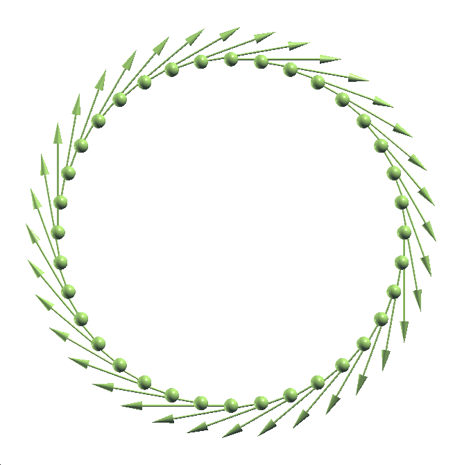
Fig. 13 Spin texture for band 235 of the Bi2Se3 multilayer

Fig. 14 Spin texture for band 236 of the Bi2Se3 multilayer